Chapter 2 Fig 3
2.1 3B: stacked bar chart.
library(tidyverse)
library(vdbR)
library(ggpubr)
connect_database('~/dbConfig.txt')
get_table_from_database("asv_annotation_blast_color_ag");
# my table of the CART stool cohort
stb <- read_csv('data/amplicon/stool/combined_2_meta.csv')
# get the counts from database and also the color for the asv
counts_data <- get_counts_subset(stb$sampleid)dat <- counts_data %>%
select(asv_key:count_total, count_relative) %>%
left_join(asv_annotation_blast_color_ag %>%
select(asv_key,color_label_group_distinct), by = "asv_key")
# there are some ASVs that don't have a color with it, but can use the color for the genus level
color_group <- dat %>%
split(is.na(.$color_label_group_distinct))
# find the genus for these asv
get_table_from_database('asv_annotation_blast_ag')
no_color <- color_group %>%
pluck('TRUE') %>%
distinct(asv_key) %>%
inner_join(asv_annotation_blast_ag %>%
select(asv_key, genus))
# find the colors for these genera
genera_colors <- no_color %>%
distinct(genus) %>%
inner_join(asv_annotation_blast_color_ag %>%
distinct(genus, color_label_group_distinct))
# the full df for the no color genera
no_color_df <- no_color %>%
left_join(genera_colors)
no_color_df_full <- color_group %>%
pluck('TRUE') %>%
select(-color_label_group_distinct) %>%
left_join(no_color_df %>%
select(- genus))
# so if the genus is unknown then it's gonna be assigned "other" gray color
# the question is do we go one taxa level higher or make a new color base and shades for the new asv
# after discussing with Tsoni, we decided that it's ok to assign gray to the unknown genus
# merge the new no_color_df_full to the original df
dat <- bind_rows(
no_color_df_full,
color_group %>%
pluck('FALSE')
)
dat %>% write_csv('data/the_data_to_make_panel_B.csv')# the color palette (inherited from Ying, used in lots of project in our lab, the palette used in the NEJM paper Fig 2D https://www.nejm.org/doi/full/10.1056/NEJMoa1900623)
asv_color_set <- asv_annotation_blast_color_ag %>%
distinct(color,color_label_group_distinct,color_label_group,color_base) %>%
select(color_label_group_distinct, color) %>%
deframe()# calculate the beta diversity between the samples which deicide the order of the samples in the plot
cbd <- compute_beta_diversity_and_tsne(sampleid = dat$sampleid,
taxonomy = dat$color_label_group_distinct,
count = dat$count);
#compute beta diversity
cbd$compute_beta_diversity()## Time:Composition_matrix:
## Time difference of 0.009665012 secs
## Time:Bray-Curtis matrix:
## Time difference of 0.00253582 secs#get beta diversity
d_beta <- cbd$get_betadiversity()
#compute hierarchical cluster
hc <- hclust(as.dist(d_beta), method = 'complete')
dend <- as.dendrogram(hc)
sample_dendogram_order <- labels(dend)
# dividing the samples to lower and higher diversity
div_order <- stb %>%
arrange(simpson_reciprocal) %>%
pull(sampleid)
###
# how about splitting the above dendrogram order into the low and higher diversity groups
div_med <- median(stb$simpson_reciprocal)
lower_samp <- stb %>%
filter(simpson_reciprocal <= div_med) %>%
pull(sampleid)
lower_samp_o <- sample_dendogram_order[sample_dendogram_order %in% lower_samp]
higher_samp_o <- sample_dendogram_order[!sample_dendogram_order %in% lower_samp]
dat$sampleid = factor(dat$sampleid,levels = c(lower_samp_o, higher_samp_o))
stacked_bar <- ggplot(dat,aes(sampleid, count_relative, fill = color_label_group_distinct) ) +
geom_bar(stat = "identity", position="fill", width = 1) +
theme_classic() +
labs(title = '',
ylab = 'Relative counts') +
theme(axis.text.x = element_text(angle = 90),
axis.text.y = element_blank(),
legend.position = "none") +
scale_fill_manual(values = asv_color_set)
stacked_bar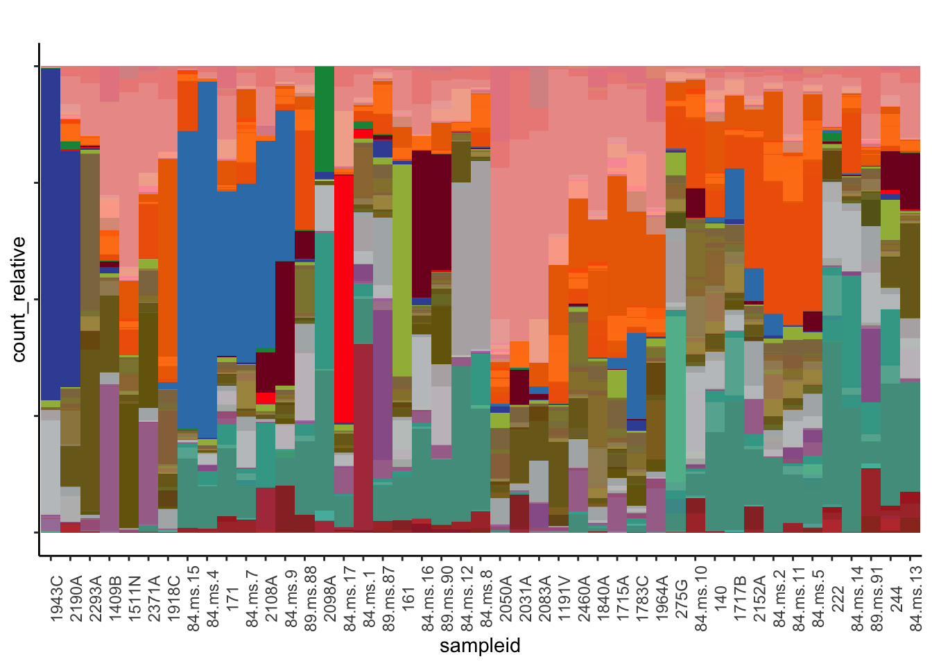
ggsave('figs/amplicon/stacked_bar_sorted_with_hclust_lower_and_higher_diversity.pdf', plot = stacked_bar,
       width = 7, height = 5)
2.2 3C: alpha and beta diversity between CART patients and healthy volunteers
2.2.1 alpha diversity (Simpson’s reciprocal)
library(vdbR)
connect_database('~/dbConfig.txt')
get_table_from_database("healthy_volunteers_ag")
get_table_from_database("asv_alpha_diversity_ag")
## [1] "table asv_alpha_diversity_ag is loaded and filtered for duplicates. Only the replicate of highest coverage is retained."# a total of 75 samples
alpha <- bind_rows(
stb %>% select(sampleid, simpson_reciprocal) %>% mutate(grp = 'baseline_CART'),
asv_alpha_diversity_ag %>%
select(sampleid, simpson_reciprocal) %>%
inner_join(healthy_volunteers_ag %>% select(sampleid), by = "sampleid") %>%
mutate(grp = 'healthy')
) %>%
distinct(sampleid, .keep_all = T)
alpha %>%
ggboxplot(x = 'grp', y = 'simpson_reciprocal', add = 'jitter',
title = '', ylab = 'Fecal diversity (Simpson Reciprocal)', xlab = '',
palette = c('#ED0000','#00468B')) +
stat_compare_means(comparisons= list(c('healthy', 'baseline_CART')),
label= "p.format",
method= 'wilcox.test')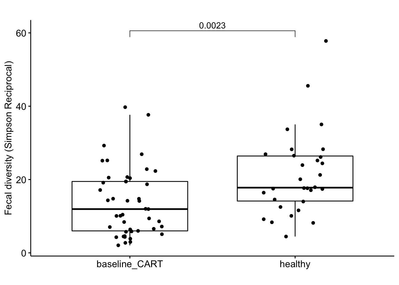
2.2.2 beta diversity (PCOA of Bray-Curtis)
PCOA of Bray-Curtis distance with counts matrix at ASV level using an abundannce threshold of 0.01% and a prevalence threshold of 25% between healthy and CART cohort.
library(vdbR)
connect_database('~/dbConfig.txt')

healthy <- healthy_volunteers_ag %>%
  inner_join(asv_alpha_diversity_ag, by = c("sampleid", "oligos_id"))
cts <- get_counts_subset(c(stb$sampleid, healthy %>% pull(sampleid)))

# a total of 75 samples counts. there are 3 healthy samples I don't have count .
nsamp <- cts %>%
  distinct(sampleid) %>%
  nrow

all_pheno <- bind_rows(healthy %>%
  select(sampleid) %>%
  mutate(grp = 'healthy', center = 'healthy'),
  stb %>% select(sampleid, center)  %>%
    mutate(grp = 'CART') %>%
    select(sampleid, grp, center)
  ) %>%
  ungroup %>%
  distinct(sampleid, .keep_all = T) %>%
  inner_join(asv_alpha_diversity_ag %>%
               distinct(sampleid, .keep_all = T) %>%
               distinct(path_pool, sampleid))


# filter >0.01% in more than 25% samples
keepa <- cts %>%
  filter(count_relative > 0.0001) %>%
  count(asv_key) %>%
  filter(n > floor(nsamp * 0.25)) %>%
  pull(asv_key)

cts_fil <- cts %>%
  filter(asv_key %in% keepa) %>%
  select(sampleid, asv_key,count_relative ) %>%
  spread(key = 'asv_key', value = 'count_relative', fill = 0) %>%
  column_to_rownames('sampleid')

library(vegan)
dist_ <- vegdist(cts_fil, method = 'bray')
eigen <- pcoa(dist_)$values$Eigenvalues
percent_var <- signif(eigen/sum(eigen), 3)*100

bc <- cmdscale(dist_, k = 2)

pcoa_two <- bc %>%
  as.data.frame() %>%
  rownames_to_column('sampleid') %>%
  ungroup() %>%
  inner_join(all_pheno) %>%
  distinct() %>%
  ggscatter(x = 'V1', y = 'V2', color =  'grp') +
  labs(title = 'PCOA of healthy and CART patients') +
  xlab(paste0("PC 1 [",percent_var[1],"%]")) +
  ylab(paste0("PC 2 [",percent_var[2],"%]"))
  #theme_void() +

pcoa_two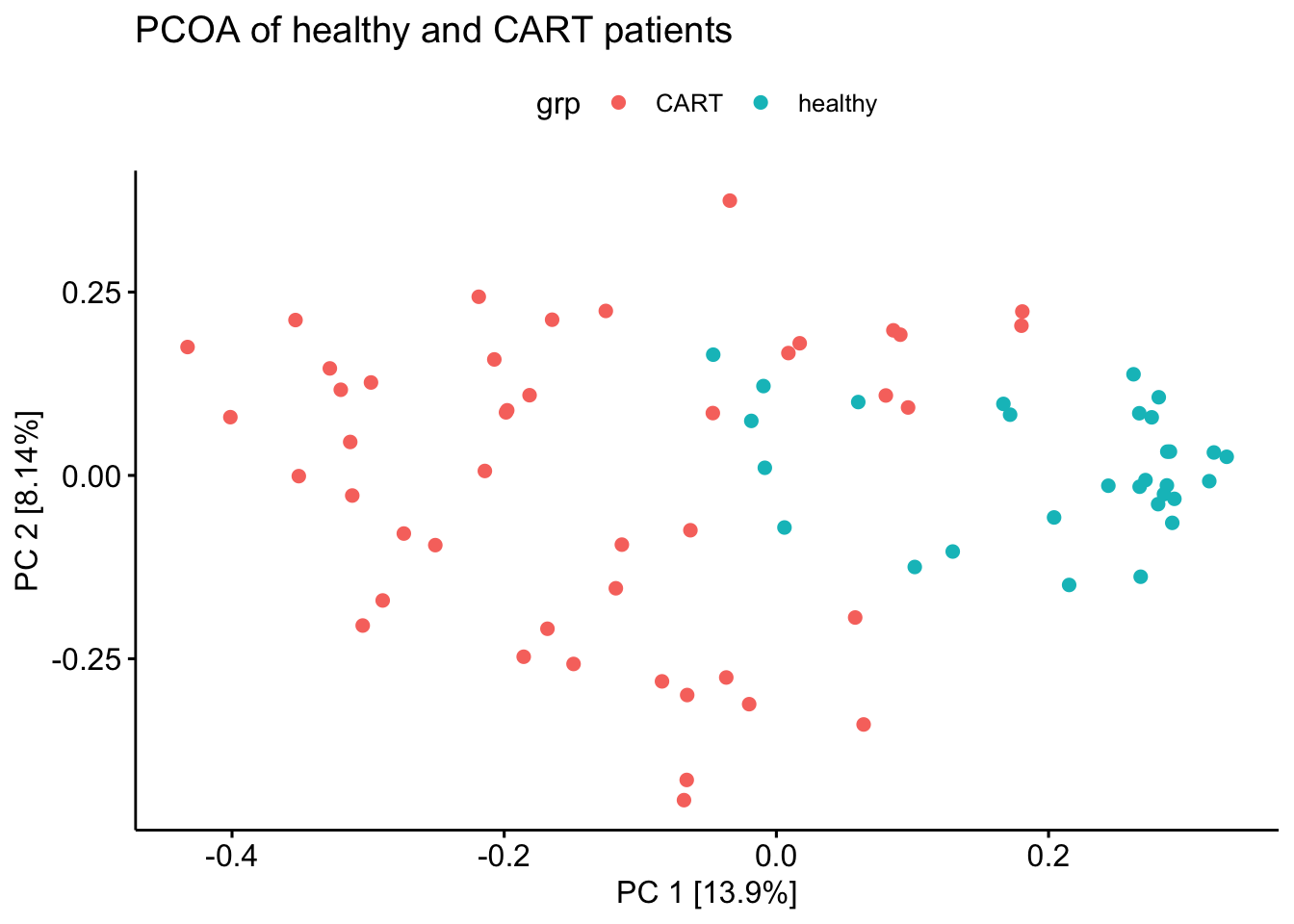
ggsave('figs/PCOA(bray-curtis) of healthy and CART patients.pdf', plot = pcoa_two)The PCOA with only CART patients data using the same filtering threshold but colored with the different pools they are sequenced from.
# a pcoa at asv level to show they are from different pools and well mixed
cts <- get_counts_subset(c(stb$sampleid))

# filter >0.01% in more than 25% samples
keepa <- cts %>%
  filter(count_relative > 0.0001) %>%
  count(asv_key) %>%
  filter(n > floor(nsamp * 0.25)) %>%
  pull(asv_key)

cts_fil <- cts %>%
  filter(asv_key %in% keepa) %>%
  select(sampleid, asv_key,count_relative ) %>%
  spread(key = 'asv_key', value = 'count_relative', fill = 0) %>%
  column_to_rownames('sampleid')

dist_ <- vegdist(cts_fil, method = 'bray')
eigen <- pcoa(dist_)$values$Eigenvalues
percent_var <- signif(eigen/sum(eigen), 3)*100

bc <- cmdscale(dist_, k = 2)

mp <- bc %>%
  as.data.frame() %>%
  rownames_to_column('sampleid') %>%
  ungroup() %>%
  inner_join(all_pheno) %>%
  distinct(sampleid, .keep_all = T)  %>%
  mutate(pool = str_extract(path_pool, 'Sample.+/')) %>%
  mutate(pool = str_replace(pool, 'Sample_','')) %>%
  mutate(pool = if_else(str_detect(pool, 'IGO'), str_extract(pool, 'IGO.+$'), pool)) %>%
  mutate(pool = str_replace(pool, '_1/|_comple.+$',''))

pcoa_cart <- mp %>%
  ggscatter(x = 'V1', y = 'V2', color =  'pool', size = 3) +
  labs(title = 'PCOA of CART patients') +
  xlab(paste0("PC 1 [",percent_var[1],"%]")) +
  ylab(paste0("PC 2 [",percent_var[2],"%]"))
  #theme_void() +

pcoa_cart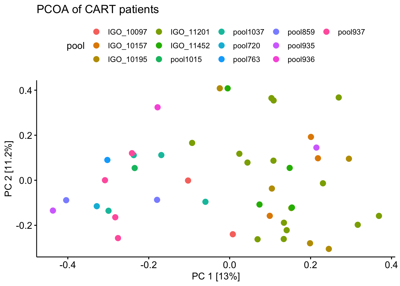
ggsave('figs/PCOA(bray-curtis) (ASV level)of CART patients_pool.pdf', width = 9, height = 9, plot = pcoa_cart)2.3 Fig 3 E&F Lefse analysis with taxa abundance at ASV level
library(tidyverse)
library(ggpubr)
# sort out the asv counts table and also do filtering (need to have all taxa levels)
meta <- read_csv('data/amplicon/stool/combined_2_meta.csv')
library(vdbR)
connect_database('~/dbConfig.txt')
get_table_from_database('asv_annotation_blast_ag')
cts <- get_counts_subset(meta$sampleid)
cts_ <- cts %>%
select(asv_key, sampleid, count_relative) %>%
spread(key = 'sampleid', value = 'count_relative', fill = 0)
annot <- asv_annotation_blast_ag %>%
filter(asv_key %in% cts_$asv_key) %>%
mutate(ordr = if_else(is.na(ordr), str_glue('unknown_of_class_{class}'), ordr),
family = if_else(is.na(family), str_glue('unknown_of_order_{ordr}'), family),
genus = if_else(is.na(genus) , str_glue('unknown_of_family_{family}'), genus),
species = if_else(is.na(species) , str_glue('unknown_of_genus_{genus}'), species)) %>%
mutate(taxa_asv = str_glue('k__{kingdom}|p__{phylum}|c__{class}|o__{ordr}|f__{family}|g__{genus}|s__{species}|a__{asv_key}'))
cts_all <- cts_ %>%
full_join(annot %>% select(asv_key, taxa_asv), by = 'asv_key') %>%
select(-asv_key) %>%
gather('sampleid', 'relab', names(.)[1]:names(.)[ncol(.)-1]) %>%
left_join(meta %>% select(sampleid, cr_d100, toxicity), by = 'sampleid')
# the asv to keep
# keep the asvs that show up in at least 25% of the samples
keepg <- cts_all %>%
filter(relab > 0.0001) %>%
ungroup() %>%
count(taxa_asv) %>%
filter(n > floor(nrow(meta) * 0.25)) %>%
pull(taxa_asv)
cts_fil <- cts_all %>%
filter(taxa_asv %in% keepg) %>%
spread('sampleid', 'relab', fill = 0)# the pheno label for the samples
pheno <- meta %>%
select(center, cr_d100:crs, icans, sampleid) %>%
gather('pheno', 'value', cr_d100:icans)
all_sub_pheno <- pheno %>%
split(., list(.$pheno)) %>%
purrr::imap(~ filter(.data = ., value != 'not_assessed'))
tpheno <- all_sub_pheno %>%
imap(function(.x, .y){
select(.data = .x, value) %>%
t() %>% write.table(str_glue('data/amplicon/lefse/pull_{.y}.txt'), sep = '\t', quote = F, row.names = T, col.names = F)
})
tcts <- all_sub_pheno %>%
purrr::map(~ pull(.data = ., sampleid) ) %>%
imap(~ cts_fil %>% select(taxa_asv, matches(.x)) %>% write_tsv(str_glue('data/amplicon/lefse/{.y}_asv_tcts.tsv'))) cat data/amplicon/lefse/pull_toxicity.txt data/amplicon/lefse/toxicity_asv_tcts.tsv > data/amplicon/lefse/pull_toxicity_asv_tcts.tsv
cat data/amplicon/lefse/pull_cr_d100.txt data/amplicon/lefse/cr_d100_asv_tcts.tsv > data/amplicon/lefse/pull_cr_d100_asv_tcts.tsv fns <- list.files('data/amplicon/lefse/', pattern = 'pull.*_asv_tcts.tsv$')
cmds <- tibble(
fns = fns
) %>%
mutate(format_cmd = str_glue('lefse_format_input.py {fns} {fns}.in -c 1 -u 2 -o 1000000 ')) %>%
mutate(run_cmd = str_glue('lefse_run.py -l 4 {fns}.in {fns}.res')) %>%
mutate(plot_cmd = str_glue('lefse_plot_res.py {fns}.res {fns}.pdf --format pdf --feature_font_size 4 --width 10 --dpi 300 --title {fns}')) %>%
mutate(clado_cmd = str_glue('lefse_plot_cladogram.py {fns}.res {fns}_clado.pdf --label_font_size 4 --dpi 300 --format pdf --title {fns}')) %>%
select(-fns) %>%
gather() %>%
select(value) %>%
write_csv('data/amplicon/lefse/lefse_run_cmd_taxa.sh', col_names = F)# run in terminal:
# bash /Users/daia1/projects/CART_and_microbiome/data/amplicon/lefse/lefse_run_cmd_taxa.sh# visualize the results in ggplot
# the input : lefse res files
fns <- list.files('data/amplicon/lefse/', pattern = 'pull.*_asv_tcts.tsv.res$', full.names = T)
# join all of the tables feature together
feature <- fns %>%
set_names(fns) %>%
purrr::map(~ read_tsv(., col_names = c('feature','xx','direction','score','pval')) %>%
filter(!is.na(score))) %>%
bind_rows(.id = 'group') %>%
mutate(group = str_replace(group, 'data/amplicon/lefse//pull_','')) %>%
mutate(group = str_replace(group, '_asv_tcts.tsv.res$',''))
# change the "N" direction to be minus score
feature <- bind_rows(
feature %>%
split(.$direction) %>%
pluck('no') %>%
mutate(score = -score),
feature %>%
split(.$direction) %>%
pluck('yes')
) %>%
arrange(group, feature, score) %>%
mutate(feature = str_replace_all(feature, '^.+\\.', ''))
all_title_fs <- 20
axis_text_fs <- 16
CR <- feature %>%
filter(group == 'cr_d100') %>%
ggplot(aes(x = reorder(feature, score), y = score, fill = direction)) +
geom_bar( stat = 'identity') +
coord_flip() +
scale_color_manual(values = c('#925E9F', '#42B540')) +
scale_fill_manual(values = c('#925E9F', '#42B540')) +
theme_classic() +
theme(axis.title.y = element_blank(),
plot.title = element_text(size=all_title_fs),
axis.title.x = element_text(size=axis_text_fs),
axis.text.x = element_text(size=axis_text_fs),
legend.position='bottom') +
labs(title = str_glue('Response to CR') ,
y = 'Score')
CR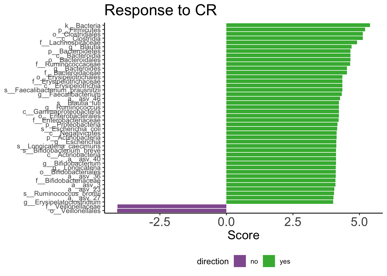
tox <- feature %>%
  filter(group == 'toxicity') %>%
  ggplot(aes(x = reorder(feature, score), y = score, fill = direction)) +
            geom_bar(stat = 'identity') +
            coord_flip() +
            scale_color_manual(values = c('#0099B4', '#AD002A'))  +
            scale_fill_manual(values = c('#0099B4', '#AD002A')) +
            theme_classic() +
            theme(axis.title.y  = element_blank(),
                  axis.title.x = element_text(size=axis_text_fs),
                  plot.title = element_text(size=all_title_fs),
                  axis.text.x = element_text(size=axis_text_fs),
                  legend.position="bottom") +
            labs(title = str_glue('Response to Toxicity') ,
                 y = 'Score')

tox
g <- cowplot::plot_grid(CR,tox,
          nrow = 2,
          align = 'hv',
          rel_heights = c(1.8,1.2),
          axis = 'b')
g
ggsave('figs/amplicon/16s_lefse_combined.pdf', device = 'pdf', height = 15, width = 15, plot = g)


ggsave('figs/amplicon/16s_lefse_tox.pdf', device = 'pdf', height = 10, width = 10, plot = tox)

ggsave('figs/amplicon/16s_lefse_CR.pdf', device = 'pdf', height = 10, width = 10, plot = CR)
It is important to check the relative abundance of the significant taxa visually.
# to see the relative abundance of those taxa
# to get the top and bottom three taxa of the lefse results
res <- list.files('data/amplicon/lefse/', pattern = 'asv_tcts.tsv.res$', full.names = T)

# gather the species level taxa in the lefse significant results
res_all <- res %>%
  set_names(res) %>%
  purrr::map(~ read_tsv(., col_names = c('feature','xx','direction','score','pval')) %>%
        filter(!is.na(score))) %>%
  keep(~ nrow(.) > 0) %>%
  bind_rows(.id = 'res') %>%
  mutate(res = str_replace(res, '^.+//',''),
         res = str_replace(res, '_asv.+$',''))  %>%
  rename(grp = res) %>%
  filter(grp %in% c('pull_cr_d100','pull_toxicity')) %>%
  mutate(feature = str_replace_all(feature, '\\.','\\|')) %>%
  #split(., list(.$grp, .$direction)) %>%
  #map_dfr(~ top_n(x = ., n = 4, wt = score) %>% arrange(-score)) %>%
  # filter(str_detect(feature, 's__.+$')) %>%
  # filter(!str_detect(feature, 'a__.+$')) %>%
  filter(str_detect(feature, 'g__.+$')) %>%
  filter(!str_detect(feature, 's__.+$')) %>%
  mutate(feature = str_replace(feature, '^.+g__','')) %>%
  mutate(feature = str_replace(feature, '_Clostridium_', '[Clostridium]')) %>%
  ungroup()


# plot the relab of those taxa (at species level) in boxplot
# get the species counts of the sampels
cts_spp <- cts_ %>%
  full_join(annot %>%  select(asv_key, species), by  = 'asv_key') %>%
  select(-asv_key)  %>%
  gather('sampleid', 'relab', names(.)[1]:names(.)[ncol(.)-1]) %>%
  group_by(sampleid, species) %>%
  summarise(Relab = sum(relab)) %>%
  select(sampleid, species, Relab) %>%
  left_join(meta %>% select(sampleid, cr_d100, toxicity), by = 'sampleid') %>%
  ungroup()

cts_genus <- cts_ %>%
  full_join(annot %>%  select(asv_key, genus), by  = 'asv_key') %>%
  select(-asv_key)  %>%
  gather('sampleid', 'relab', names(.)[1]:names(.)[ncol(.)-1]) %>%
  group_by(sampleid, genus) %>%
  summarise(Relab = sum(relab)) %>%
  select(sampleid, genus, Relab) %>%
  left_join(meta %>% select(sampleid, cr_d100, toxicity), by = 'sampleid') %>%
  ungroup()

joined <- cts_genus %>%
  inner_join(res_all, by = c('genus' = 'feature'))

# finally I can do the plotting

pull_cr_d100 <- joined  %>%
  filter(grp == 'pull_cr_d100') %>%
  ggboxplot(x = 'cr_d100', y = 'Relab', add = 'jitter', title = 'Outcome: cr_d100') +
  facet_wrap(direction ~ genus, scales="free_y")
pull_cr_d100 
ggsave('figs/amplicon/lefse_taxa_crd100.pdf', width = 15, height = 13, plot = pull_cr_d100)As can be observed in the boxplot, patients that had a CR have higher median relative abundance in Ruminococcus.
pull_toxicity <- joined  %>%
  filter(grp == 'pull_toxicity') %>%
  ggboxplot(x = 'toxicity', y = 'Relab', add = 'jitter', title = 'Outcome: toxicity') +
  facet_wrap(direction ~ genus, scales="free_y")
pull_toxicity 
ggsave('figs/amplicon/lefse_taxa_toxicity.pdf', width = 15, height = 13, plot = pull_toxicity)As can be observed in the boxplot, patients that had a toxicity response have clearly higher median relative abundance in Bacteroides.
# to do the wilcoxn test per taxa annd then p-adjust
df <- joined %>%
  filter(genus == 'Bacteroides' & grp == 'pull_cr_d100')

    test =wilcox.test(df %>% filter(cr_d100 == 'yes') %>% pull(Relab), df %>% filter(cr_d100 == 'no') %>% pull(Relab))
## Warning in wilcox.test.default(df %>% filter(cr_d100 == "yes") %>%
## pull(Relab), : cannot compute exact p-value with ties test$p.value## [1] 0.9728295cr_res <- joined %>%
filter(grp == 'pull_cr_d100') %>%
split(.$genus) %>%
imap_dfr(function(.x, .y){
test =wilcox.test(.x %>% filter(cr_d100 == 'yes') %>% pull(Relab), .x %>% filter(cr_d100 == 'no') %>% pull(Relab), exact = F)
return(test$p.value)
}) %>%
gather() %>%
rename(pval = value) %>%
mutate(padj = p.adjust(pval, method = 'BH')) %>%
mutate(grp = 'pull_cr_d100')
tox_res <- joined %>%
filter(grp == 'pull_toxicity') %>%
split(.$genus) %>%
imap_dfr(function(.x, .y){
test =wilcox.test(.x %>% filter(toxicity == 'yes') %>% pull(Relab), .x %>% filter(toxicity == 'no') %>% pull(Relab), exact = F)
return(test$p.value)
}) %>%
gather() %>%
rename(pval = value) %>%
mutate(padj = p.adjust(pval, method = 'BH')) %>%
mutate(grp = 'pull_toxicity')
all <- bind_rows(cr_res, tox_res)
all %>%
write_csv('data/lefse_sig_taxa_padj.csv')2.4 Fig 3D Bayesian modeling with microbiome alpha diversity as predictor
The formular is: CR/Toxicity ~ alpha diversity + center
library(tidyverse)
library(ggpubr)
library(rethinking)
library(tidybayes)
options(mc.cores = parallel::detectCores())

meta <- read_csv('data/amplicon/stool/combined_2_meta.csv') %>%
  mutate(logdiv_s = scale(log(simpson_reciprocal))) %>%
  mutate(logdiv_s = as.numeric(logdiv_s)) %>%
  mutate(tox = if_else(toxicity == 'yes', 1, 0),
         cr100 = if_else(cr_d100 == 'yes', 1, 0),
         loca = if_else(center == 'M', 1, 2)) %>%  # MSK 1 ; Upenn 2
  mutate(center = factor(center),
         toxicity = factor(toxicity, levels = c('no','yes')),
         cr_d100 = factor(cr_d100, levels = c('no','yes')))

meta %>% readr::write_csv('data/amplicon/stool/combined_2_meta_expanded.csv')

set.seed(123)
dat_list <- list(
    tox = meta$tox,
    crs3 = meta$crs3,
    cr100 = meta$cr100,
    location = meta$loca,
    logdiv_s = meta$logdiv_s
    )
## Warning: Unknown or uninitialised column: `crs3`.2.4.1 outcome: toxicity
mtox <- ulam(
    alist(
        tox ~ dbinom( 1 , p ) ,
        logit(p) <- b*logdiv_s + a[location] ,
        b ~ dnorm( 0 , 2),
        a[location] ~ dnorm( 0 , 0.5 )
    ) , data=dat_list , chains=4 , log_lik=TRUE , cores = 16)
## Running /Library/Frameworks/R.framework/Resources/bin/R CMD SHLIB foo.c
## clang -mmacosx-version-min=10.13 -I"/Library/Frameworks/R.framework/Resources/include" -DNDEBUG -I"/Library/Frameworks/R.framework/Versions/4.1/Resources/library/Rcpp/include/" -I"/Library/Frameworks/R.framework/Versions/4.1/Resources/library/RcppEigen/include/" -I"/Library/Frameworks/R.framework/Versions/4.1/Resources/library/RcppEigen/include/unsupported" -I"/Library/Frameworks/R.framework/Versions/4.1/Resources/library/BH/include" -I"/Library/Frameworks/R.framework/Versions/4.1/Resources/library/StanHeaders/include/src/" -I"/Library/Frameworks/R.framework/Versions/4.1/Resources/library/StanHeaders/include/" -I"/Library/Frameworks/R.framework/Versions/4.1/Resources/library/RcppParallel/include/" -I"/Library/Frameworks/R.framework/Versions/4.1/Resources/library/rstan/include" -DEIGEN_NO_DEBUG -DBOOST_DISABLE_ASSERTS -DBOOST_PENDING_INTEGER_LOG2_HPP -DSTAN_THREADS -DBOOST_NO_AUTO_PTR -include '/Library/Frameworks/R.framework/Versions/4.1/Resources/library/StanHeaders/include/stan/math/prim/mat/fun/Eigen.hpp' -D_REENTRANT -DRCPP_PARALLEL_USE_TBB=1 -I/usr/local/include -fPIC -Wall -g -O2 -c foo.c -o foo.o
## In file included from <built-in>:1:
## In file included from /Library/Frameworks/R.framework/Versions/4.1/Resources/library/StanHeaders/include/stan/math/prim/mat/fun/Eigen.hpp:13:
## In file included from /Library/Frameworks/R.framework/Versions/4.1/Resources/library/RcppEigen/include/Eigen/Dense:1:
## In file included from /Library/Frameworks/R.framework/Versions/4.1/Resources/library/RcppEigen/include/Eigen/Core:88:
## /Library/Frameworks/R.framework/Versions/4.1/Resources/library/RcppEigen/include/Eigen/src/Core/util/Macros.h:628:1: error: unknown type name 'namespace'
## namespace Eigen {
## ^
## /Library/Frameworks/R.framework/Versions/4.1/Resources/library/RcppEigen/include/Eigen/src/Core/util/Macros.h:628:16: error: expected ';' after top level declarator
## namespace Eigen {
## ^
## ;
## In file included from <built-in>:1:
## In file included from /Library/Frameworks/R.framework/Versions/4.1/Resources/library/StanHeaders/include/stan/math/prim/mat/fun/Eigen.hpp:13:
## In file included from /Library/Frameworks/R.framework/Versions/4.1/Resources/library/RcppEigen/include/Eigen/Dense:1:
## /Library/Frameworks/R.framework/Versions/4.1/Resources/library/RcppEigen/include/Eigen/Core:96:10: fatal error: 'complex' file not found
## #include <complex>
## ^~~~~~~~~
## 3 errors generated.
## make: *** [foo.o] Error 1# make the forest plot
df <- precis(mtox, prob = 0.95) %>% as.tibble()## Warning: `as.tibble()` was deprecated in tibble 2.0.0.
## Please use `as_tibble()` instead.
## The signature and semantics have changed, see `?as_tibble`.df <- df %>%
mutate(variable = 'simpson_reciprocal')
#remove row number 1 (The intercept)
forest <- df %>%
ggplot(aes(x = reorder(variable, mean), y = mean)) +
geom_point(shape = 15,
size = 4, width = 0.1,
position = "dodge", color="black") +
geom_errorbar(aes(ymin = `2.5%`,
ymax = `97.5%`),
width = 0.1,
size = 0.7,
position = "dodge", color="turquoise4") +
theme(axis.title = element_text(face = "bold")) +
#xlab("Variables") + ylab("Coefficient with 95% CI") +
coord_flip(ylim = c(-0.7, 1)) +
geom_hline(yintercept = 0, color = "red", size = 1) +
theme(axis.title = element_text(size = 0)) +
theme(axis.text = element_text(size = 14)) +
labs(title = '95% confidence interval of the coefficients\nfor standardized log transformed alpha diversity when outcome is toxicity',
x = '',
y = 'Association with Toxicity') ## Warning: Ignoring unknown parameters: widthforest ## Warning: Width not defined. Set with `position_dodge(width = ?)`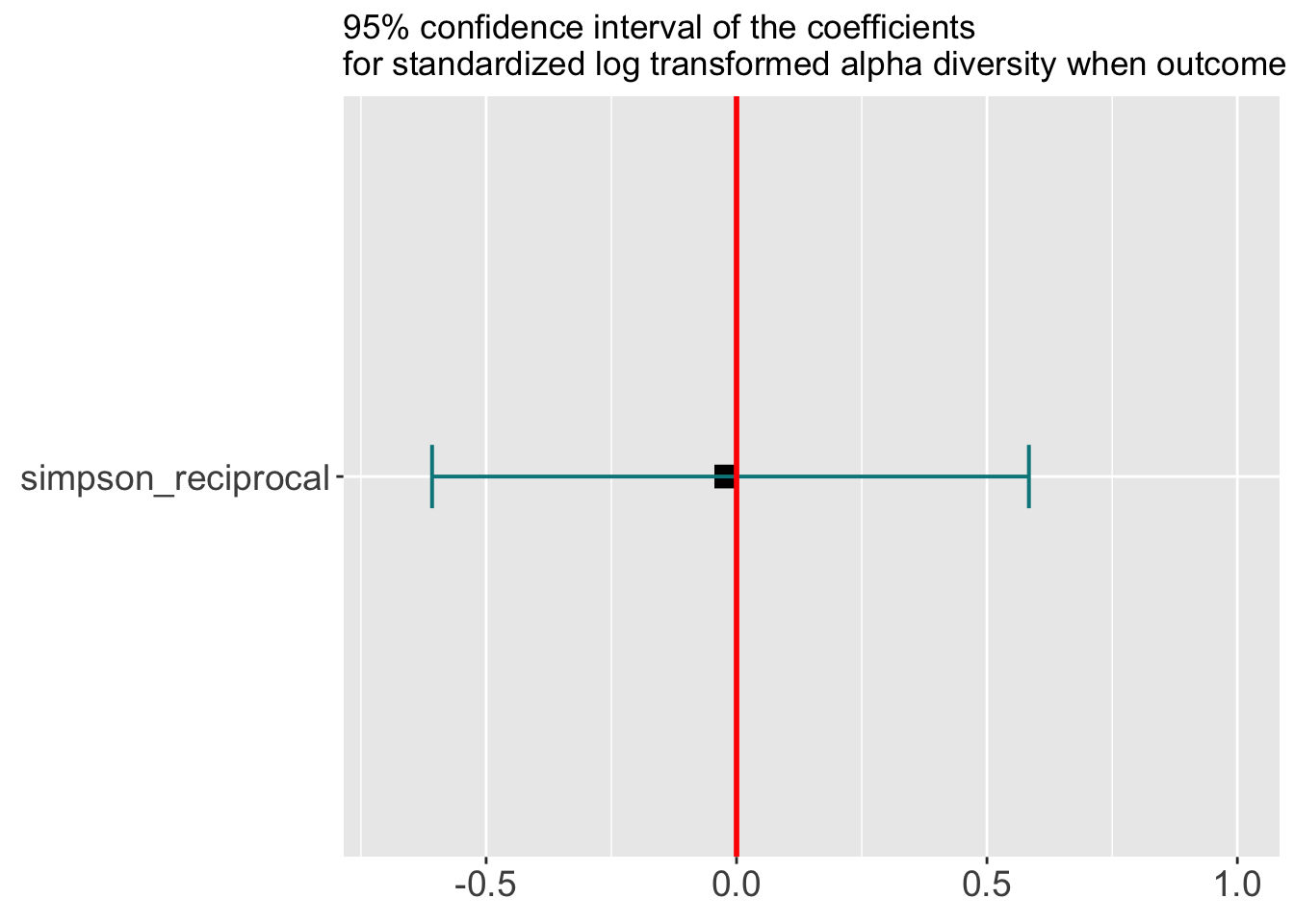
ggsave('figs/amplicon/bayesian_div_tox.pdf', width = 5, height = 4, plot = forest)## Warning: Width not defined. Set with `position_dodge(width = ?)`To examine the diversity’s correlation with the toxicity response, imagine there are two hypothetical patients, with diversity of -1 and 1 on the transformed scale for simpson reciprocal diversity, representing “low” and “high” diversity scenarios. We want to see what is the difference between predicted probability of havinng a toxicity response when the diversity is “low” and "“high” in before seeing the data (prior) and after seeing the data (posterior) situations.
set.seed(123)
library(tidybayes)
theme_set(theme_tidybayes() + cowplot::panel_border())
div_value <- c(-1, 1)
# prior check: the differennce in probability
prior <- extract.prior( mtox , n=4000 )
## Running /Library/Frameworks/R.framework/Resources/bin/R CMD SHLIB foo.c
## clang -mmacosx-version-min=10.13 -I"/Library/Frameworks/R.framework/Resources/include" -DNDEBUG -I"/Library/Frameworks/R.framework/Versions/4.1/Resources/library/Rcpp/include/" -I"/Library/Frameworks/R.framework/Versions/4.1/Resources/library/RcppEigen/include/" -I"/Library/Frameworks/R.framework/Versions/4.1/Resources/library/RcppEigen/include/unsupported" -I"/Library/Frameworks/R.framework/Versions/4.1/Resources/library/BH/include" -I"/Library/Frameworks/R.framework/Versions/4.1/Resources/library/StanHeaders/include/src/" -I"/Library/Frameworks/R.framework/Versions/4.1/Resources/library/StanHeaders/include/" -I"/Library/Frameworks/R.framework/Versions/4.1/Resources/library/RcppParallel/include/" -I"/Library/Frameworks/R.framework/Versions/4.1/Resources/library/rstan/include" -DEIGEN_NO_DEBUG -DBOOST_DISABLE_ASSERTS -DBOOST_PENDING_INTEGER_LOG2_HPP -DSTAN_THREADS -DBOOST_NO_AUTO_PTR -include '/Library/Frameworks/R.framework/Versions/4.1/Resources/library/StanHeaders/include/stan/math/prim/mat/fun/Eigen.hpp' -D_REENTRANT -DRCPP_PARALLEL_USE_TBB=1 -I/usr/local/include -fPIC -Wall -g -O2 -c foo.c -o foo.o
## In file included from <built-in>:1:
## In file included from /Library/Frameworks/R.framework/Versions/4.1/Resources/library/StanHeaders/include/stan/math/prim/mat/fun/Eigen.hpp:13:
## In file included from /Library/Frameworks/R.framework/Versions/4.1/Resources/library/RcppEigen/include/Eigen/Dense:1:
## In file included from /Library/Frameworks/R.framework/Versions/4.1/Resources/library/RcppEigen/include/Eigen/Core:88:
## /Library/Frameworks/R.framework/Versions/4.1/Resources/library/RcppEigen/include/Eigen/src/Core/util/Macros.h:628:1: error: unknown type name 'namespace'
## namespace Eigen {
## ^
## /Library/Frameworks/R.framework/Versions/4.1/Resources/library/RcppEigen/include/Eigen/src/Core/util/Macros.h:628:16: error: expected ';' after top level declarator
## namespace Eigen {
## ^
## ;
## In file included from <built-in>:1:
## In file included from /Library/Frameworks/R.framework/Versions/4.1/Resources/library/StanHeaders/include/stan/math/prim/mat/fun/Eigen.hpp:13:
## In file included from /Library/Frameworks/R.framework/Versions/4.1/Resources/library/RcppEigen/include/Eigen/Dense:1:
## /Library/Frameworks/R.framework/Versions/4.1/Resources/library/RcppEigen/include/Eigen/Core:96:10: fatal error: 'complex' file not found
## #include <complex>
## ^~~~~~~~~
## 3 errors generated.
## make: *** [foo.o] Error 1
##
## SAMPLING FOR MODEL '28b7d1edeed92c714c94fb24d1ba3735' NOW (CHAIN 1).
## Chain 1:
## Chain 1: Gradient evaluation took 1.9e-05 seconds
## Chain 1: 1000 transitions using 10 leapfrog steps per transition would take 0.19 seconds.
## Chain 1: Adjust your expectations accordingly!
## Chain 1:
## Chain 1:
## Chain 1: Iteration: 1 / 8000 [ 0%] (Warmup)
## Chain 1: Iteration: 800 / 8000 [ 10%] (Warmup)
## Chain 1: Iteration: 1600 / 8000 [ 20%] (Warmup)
## Chain 1: Iteration: 2400 / 8000 [ 30%] (Warmup)
## Chain 1: Iteration: 3200 / 8000 [ 40%] (Warmup)
## Chain 1: Iteration: 4000 / 8000 [ 50%] (Warmup)
## Chain 1: Iteration: 4001 / 8000 [ 50%] (Sampling)
## Chain 1: Iteration: 4800 / 8000 [ 60%] (Sampling)
## Chain 1: Iteration: 5600 / 8000 [ 70%] (Sampling)
## Chain 1: Iteration: 6400 / 8000 [ 80%] (Sampling)
## Chain 1: Iteration: 7200 / 8000 [ 90%] (Sampling)
## Chain 1: Iteration: 8000 / 8000 [100%] (Sampling)
## Chain 1:
## Chain 1: Elapsed Time: 0.112933 seconds (Warm-up)
## Chain 1: 0.110755 seconds (Sampling)
## Chain 1: 0.223688 seconds (Total)
## Chain 1:prior_tox <- list(m = 1, p = 2) %>%
purrr::map(function(center_){
cols = seq(1, length(div_value)) %>%
set_names(seq(1, length(div_value))) %>%
purrr::map(function(idx){
inv_logit( prior$b * div_value[idx] + prior$a[, center_] )
})
diff = cols[[1]] -cols[[2]]
return(diff)
})
# post check: the differennce in probability
post <- extract.samples(mtox)
post_tox <- list(m = 1, p = 2) %>%
purrr::map(function(center_){
cols = seq(1, length(div_value)) %>%
set_names(seq(1, length(div_value))) %>%
purrr::map(function(idx){
inv_logit( post$b * div_value[idx] + post$a[, center_] )
})
diff = cols[[1]] -cols[[2]]
return(diff)
})
# bind the two and plot the forest plot
bind_rows(
data_frame(
coeff = c(prior_tox$m, prior_tox$p),
grp = 'prior'
),
data_frame(
coeff = c(post_tox$m, post_tox$p),
grp = 'post'
)
) %>%
ggplot(aes(x = coeff, y = grp, color = grp)) +
stat_pointinterval(.width = c(.66, .95)) +
geom_vline(xintercept = 0, col = 'gray', linetype = 'dashed')## Warning: `data_frame()` was deprecated in tibble 1.1.0.
## Please use `tibble()` instead.
- The prior and posterior confidence interval for the coefficient for scaled log transformed diversity. The median denotes median value. The thinker line represents 66% CI and the thinner line for 95% CI.
- The above figure showes that, on average, we don’t assume there is a positive or negative correlation between microbiome diversity and a response to toxicity. Thus the median is at 0. But the correlation could be big. For example, there is a probability of 1 of having a toxicity response when the diversity is low and no possibility of having a toxicity response when the diversity is high. Thus the difference in probability (blue line) could reach 1. This assumption is based on our understanding from the literature that microbiome could have big impact on immunology. See this paper (https://www.nature.com/articles/s41586-020-2971-8).
- After learning from the data, the interval shrinks in the red line, indicating we are more sure of the correlation, which is 0 since it still centers on 0.
2.4.2 outcome : CR_d100
mcr <- ulam(
    alist(
        cr100 ~ dbinom( 1 , p ) ,
        logit(p) <- b*logdiv_s + a[location] ,
        b ~ dnorm( 0 , 2),
        a[location] ~ dnorm( 0 , 0.5 )
    ) , data=dat_list , chains=4 , log_lik=TRUE , cores = 16)
## Running /Library/Frameworks/R.framework/Resources/bin/R CMD SHLIB foo.c
## clang -mmacosx-version-min=10.13 -I"/Library/Frameworks/R.framework/Resources/include" -DNDEBUG -I"/Library/Frameworks/R.framework/Versions/4.1/Resources/library/Rcpp/include/" -I"/Library/Frameworks/R.framework/Versions/4.1/Resources/library/RcppEigen/include/" -I"/Library/Frameworks/R.framework/Versions/4.1/Resources/library/RcppEigen/include/unsupported" -I"/Library/Frameworks/R.framework/Versions/4.1/Resources/library/BH/include" -I"/Library/Frameworks/R.framework/Versions/4.1/Resources/library/StanHeaders/include/src/" -I"/Library/Frameworks/R.framework/Versions/4.1/Resources/library/StanHeaders/include/" -I"/Library/Frameworks/R.framework/Versions/4.1/Resources/library/RcppParallel/include/" -I"/Library/Frameworks/R.framework/Versions/4.1/Resources/library/rstan/include" -DEIGEN_NO_DEBUG -DBOOST_DISABLE_ASSERTS -DBOOST_PENDING_INTEGER_LOG2_HPP -DSTAN_THREADS -DBOOST_NO_AUTO_PTR -include '/Library/Frameworks/R.framework/Versions/4.1/Resources/library/StanHeaders/include/stan/math/prim/mat/fun/Eigen.hpp' -D_REENTRANT -DRCPP_PARALLEL_USE_TBB=1 -I/usr/local/include -fPIC -Wall -g -O2 -c foo.c -o foo.o
## In file included from <built-in>:1:
## In file included from /Library/Frameworks/R.framework/Versions/4.1/Resources/library/StanHeaders/include/stan/math/prim/mat/fun/Eigen.hpp:13:
## In file included from /Library/Frameworks/R.framework/Versions/4.1/Resources/library/RcppEigen/include/Eigen/Dense:1:
## In file included from /Library/Frameworks/R.framework/Versions/4.1/Resources/library/RcppEigen/include/Eigen/Core:88:
## /Library/Frameworks/R.framework/Versions/4.1/Resources/library/RcppEigen/include/Eigen/src/Core/util/Macros.h:628:1: error: unknown type name 'namespace'
## namespace Eigen {
## ^
## /Library/Frameworks/R.framework/Versions/4.1/Resources/library/RcppEigen/include/Eigen/src/Core/util/Macros.h:628:16: error: expected ';' after top level declarator
## namespace Eigen {
## ^
## ;
## In file included from <built-in>:1:
## In file included from /Library/Frameworks/R.framework/Versions/4.1/Resources/library/StanHeaders/include/stan/math/prim/mat/fun/Eigen.hpp:13:
## In file included from /Library/Frameworks/R.framework/Versions/4.1/Resources/library/RcppEigen/include/Eigen/Dense:1:
## /Library/Frameworks/R.framework/Versions/4.1/Resources/library/RcppEigen/include/Eigen/Core:96:10: fatal error: 'complex' file not found
## #include <complex>
## ^~~~~~~~~
## 3 errors generated.
## make: *** [foo.o] Error 1df <- precis(mcr, prob = 0.95) %>% as.tibble()
df <- df %>%
mutate(variable = 'simpson_reciprocal')
#remove row number 1 (The intercept)
forest <- df %>%
ggplot(aes(x = reorder(variable, mean), y = mean)) +
geom_point(shape = 15,
size = 4, width = 0.1,
position = "dodge", color="black") +
geom_errorbar(aes(ymin = `2.5%`,
ymax = `97.5%`),
width = 0.1,
size = 0.7,
position = "dodge", color="turquoise4") +
theme(axis.title = element_text(face = "bold")) +
xlab("Variables") + ylab("Coefficient with 95% CI") +
coord_flip(ylim = c(-0.7, 1)) +
geom_hline(yintercept = 0, color = "red", size = 1) +
theme(axis.title = element_text(size = 0)) +
theme(axis.text = element_text(size = 14)) +
labs(title = '95% confidence interval of the coefficients\nfor standardized log transformed alpha diversity when outcome is CR') ## Warning: Ignoring unknown parameters: widthforest## Warning: Width not defined. Set with `position_dodge(width = ?)`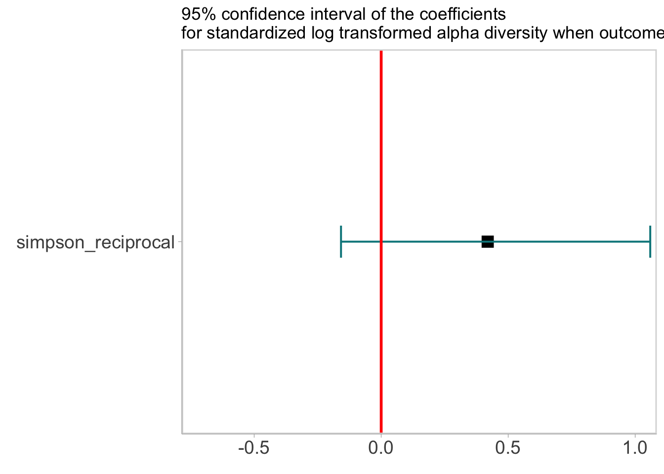
ggsave('figs/amplicon/bayesian_div_cr.pdf', width = 5, height = 4, plot = forest)## Warning: Width not defined. Set with `position_dodge(width = ?)`To examine the diversity’s correlation with the CR response, imagine there are two hypothetical patients, with diversity of -1 and 1 on the transformed scale for simpson reciprocal diversity, representing “low” and “high” diversity scenarios. We want to see what is the difference between predicted probability of havinng a CR response when the diversity is “low” and "“high” in before seeing the data (prior) and after seeing the data (posterior) situations.
set.seed(123)

# prior check: the differennce in probability
prior <- extract.prior( mcr , n=4000 )
##
## SAMPLING FOR MODEL '28b7d1edeed92c714c94fb24d1ba3735' NOW (CHAIN 1).
## Chain 1:
## Chain 1: Gradient evaluation took 1.3e-05 seconds
## Chain 1: 1000 transitions using 10 leapfrog steps per transition would take 0.13 seconds.
## Chain 1: Adjust your expectations accordingly!
## Chain 1:
## Chain 1:
## Chain 1: Iteration: 1 / 8000 [ 0%] (Warmup)
## Chain 1: Iteration: 800 / 8000 [ 10%] (Warmup)
## Chain 1: Iteration: 1600 / 8000 [ 20%] (Warmup)
## Chain 1: Iteration: 2400 / 8000 [ 30%] (Warmup)
## Chain 1: Iteration: 3200 / 8000 [ 40%] (Warmup)
## Chain 1: Iteration: 4000 / 8000 [ 50%] (Warmup)
## Chain 1: Iteration: 4001 / 8000 [ 50%] (Sampling)
## Chain 1: Iteration: 4800 / 8000 [ 60%] (Sampling)
## Chain 1: Iteration: 5600 / 8000 [ 70%] (Sampling)
## Chain 1: Iteration: 6400 / 8000 [ 80%] (Sampling)
## Chain 1: Iteration: 7200 / 8000 [ 90%] (Sampling)
## Chain 1: Iteration: 8000 / 8000 [100%] (Sampling)
## Chain 1:
## Chain 1: Elapsed Time: 0.106962 seconds (Warm-up)
## Chain 1: 0.102204 seconds (Sampling)
## Chain 1: 0.209166 seconds (Total)
## Chain 1:prior_cr <- list(m = 1, p = 2) %>%
purrr::map(function(center_){
cols = seq(1, length(div_value)) %>%
set_names(seq(1, length(div_value))) %>%
purrr::map(function(idx){
inv_logit( prior$b * div_value[idx] + prior$a[, center_] )
})
diff = cols[[1]] -cols[[2]]
return(diff)
})
# post check: the differennce in probability
post <- extract.samples(mcr)
post_cr <- list(m = 1, p = 2) %>%
purrr::map(function(center_){
cols = seq(1, length(div_value)) %>%
set_names(seq(1, length(div_value))) %>%
purrr::map(function(idx){
inv_logit( post$b * div_value[idx] + post$a[, center_] )
})
diff = cols[[1]] -cols[[2]]
return(diff)
})
# bind the two and plot the forest plot
bind_rows(
data_frame(
coeff = c(prior_cr$m, prior_cr$p),
grp = 'prior'
),
data_frame(
coeff = c(post_cr$m, post_cr$p),
grp = 'post'
)
) %>%
ggplot(aes(x = coeff, y = grp, color = grp)) +
stat_pointinterval(.width = c(.66, .95)) +
geom_vline(xintercept = 0, col = 'gray', linetype = 'dashed')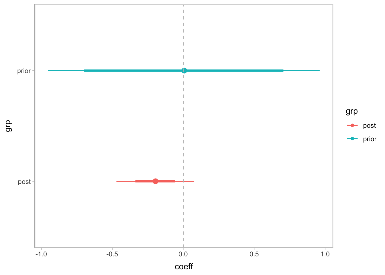
- The prior and posterior confidence interval for the coefficient for scaled log transformed diversity. The median denotes median value. The thinker line represents 66% CI and the thinner line for 95% CI.
- The above figure showes that, on average, we don’t assume there is a positive or negative correlation between microbiome diversity and a response to CR Thus the median is at 0. But the correlation could be big. For example, there is a probability of 1 of having a CR response when the diversity is low and no possibility of having a CR response when the diversity is high. Thus the difference in probability (blue line) could reach 1. This assumption is based on our understanding from the literature that microbiome could have big impact on immunology. See this paper (https://www.nature.com/articles/s41586-020-2971-8).
- After learning from the data, the interval shrinks in the red line, indicating we are more sure of the correlation. Though the 95% CI crosses 0, we are able to observe a trend of low diversity correlating to lower probability of having CR as the difference is 90% negative, suggesting a postive correlation between microbiome diversity and having a CR response.
2.5 Fig 3G Bayesian modeling with 5 genera abundance as predictor(outcome CR)
genera <- read_csv('data/amplicon/stool/combined_5_genera.csv')
# do not standardize the log transformed relative abundance
meta <- read_csv('data/amplicon/stool/combined_2_meta_expanded.csv')  %>%
  inner_join(genera)


dat_list <- list(
    tox = meta$tox,
    cr100 = meta$cr100,
    location = meta$loca,
    Akkermansia = meta$Akkermansia,
    Bacteroides = meta$Bacteroides,
    Enterococcus = meta$Enterococcus,
    Faecalibacterium = meta$Faecalibacterium,
    Ruminococcus = meta$Ruminococcus
    )
CR ~ Akkermansia + Bacteroides + Enterococcus + Faecalibacterium + Ruminococcus + center
gcr <- ulam(
    alist(
        cr100 ~ dbinom( 1 , p ) ,
        logit(p) <- ba*Akkermansia + bb*Bacteroides + be*Enterococcus + bf*Faecalibacterium + br*Ruminococcus + a[location] ,
        ba ~ dnorm( 0 , 1),
        bb ~ dnorm( 0 , 1),
        be ~ dnorm( 0 , 1),
        bf ~ dnorm( 0 , 1),
        br ~ dnorm( 0 , 1),
        a[location] ~ dnorm( 0 , 0.5 )
    ) , data=dat_list , chains=4 , log_lik=TRUE , cores = 16)
## Running /Library/Frameworks/R.framework/Resources/bin/R CMD SHLIB foo.c
## clang -mmacosx-version-min=10.13 -I"/Library/Frameworks/R.framework/Resources/include" -DNDEBUG -I"/Library/Frameworks/R.framework/Versions/4.1/Resources/library/Rcpp/include/" -I"/Library/Frameworks/R.framework/Versions/4.1/Resources/library/RcppEigen/include/" -I"/Library/Frameworks/R.framework/Versions/4.1/Resources/library/RcppEigen/include/unsupported" -I"/Library/Frameworks/R.framework/Versions/4.1/Resources/library/BH/include" -I"/Library/Frameworks/R.framework/Versions/4.1/Resources/library/StanHeaders/include/src/" -I"/Library/Frameworks/R.framework/Versions/4.1/Resources/library/StanHeaders/include/" -I"/Library/Frameworks/R.framework/Versions/4.1/Resources/library/RcppParallel/include/" -I"/Library/Frameworks/R.framework/Versions/4.1/Resources/library/rstan/include" -DEIGEN_NO_DEBUG -DBOOST_DISABLE_ASSERTS -DBOOST_PENDING_INTEGER_LOG2_HPP -DSTAN_THREADS -DBOOST_NO_AUTO_PTR -include '/Library/Frameworks/R.framework/Versions/4.1/Resources/library/StanHeaders/include/stan/math/prim/mat/fun/Eigen.hpp' -D_REENTRANT -DRCPP_PARALLEL_USE_TBB=1 -I/usr/local/include -fPIC -Wall -g -O2 -c foo.c -o foo.o
## In file included from <built-in>:1:
## In file included from /Library/Frameworks/R.framework/Versions/4.1/Resources/library/StanHeaders/include/stan/math/prim/mat/fun/Eigen.hpp:13:
## In file included from /Library/Frameworks/R.framework/Versions/4.1/Resources/library/RcppEigen/include/Eigen/Dense:1:
## In file included from /Library/Frameworks/R.framework/Versions/4.1/Resources/library/RcppEigen/include/Eigen/Core:88:
## /Library/Frameworks/R.framework/Versions/4.1/Resources/library/RcppEigen/include/Eigen/src/Core/util/Macros.h:628:1: error: unknown type name 'namespace'
## namespace Eigen {
## ^
## /Library/Frameworks/R.framework/Versions/4.1/Resources/library/RcppEigen/include/Eigen/src/Core/util/Macros.h:628:16: error: expected ';' after top level declarator
## namespace Eigen {
## ^
## ;
## In file included from <built-in>:1:
## In file included from /Library/Frameworks/R.framework/Versions/4.1/Resources/library/StanHeaders/include/stan/math/prim/mat/fun/Eigen.hpp:13:
## In file included from /Library/Frameworks/R.framework/Versions/4.1/Resources/library/RcppEigen/include/Eigen/Dense:1:
## /Library/Frameworks/R.framework/Versions/4.1/Resources/library/RcppEigen/include/Eigen/Core:96:10: fatal error: 'complex' file not found
## #include <complex>
## ^~~~~~~~~
## 3 errors generated.
## make: *** [foo.o] Error 1df <- precis(gcr, prob = 0.95) %>% as.tibble()
df <- df %>%
mutate(variable = c('Akkermansia', 'Bacteroides','Enterococcus','Faecalibacterium','Ruminococcus'))
#remove row number 1 (The intercept)
forest <- df %>%
ggplot(aes(x = variable, y = mean)) +
geom_point(shape = 15,
size = 4, width = 0.1,
position = "dodge", color="black") +
geom_errorbar(aes(ymin = `2.5%`,
ymax = `97.5%`),
width = 0.1,
size = 0.7,
position = "dodge", color="turquoise4") +
theme(axis.title = element_text(face = "bold")) +
xlab("Variables") + ylab("Coefficient with 95% CI") +
coord_flip(ylim = c(-1.5, 1.5)) +
geom_hline(yintercept = 0, color = "red", size = 1) +
theme(axis.title = element_text(size = 0)) +
theme(axis.text = element_text(size = 14)) +
labs(title = 'CR') ## Warning: Ignoring unknown parameters: widthforest ## Warning: Width not defined. Set with `position_dodge(width = ?)`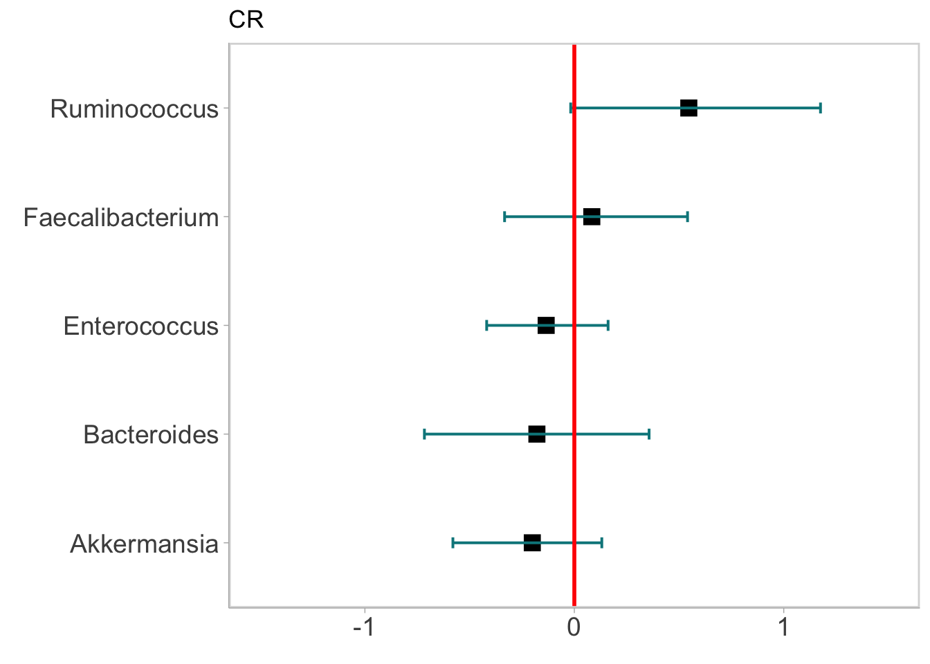
ggsave('figs/amplicon/bayesian_genera_cr_log10.pdf', width = 5, height = 4, plot = forest)## Warning: Width not defined. Set with `position_dodge(width = ?)`Check the prior and posterior coeff distribution
theme_set(theme_tidybayes() + cowplot::panel_border())
# check the prior and posterior
prior <- extract.prior( gcr , n=4000 ) %>% as.tibble()  %>% select(-a) %>% mutate(grp = 'prior')
## Running /Library/Frameworks/R.framework/Resources/bin/R CMD SHLIB foo.c
## clang -mmacosx-version-min=10.13 -I"/Library/Frameworks/R.framework/Resources/include" -DNDEBUG -I"/Library/Frameworks/R.framework/Versions/4.1/Resources/library/Rcpp/include/" -I"/Library/Frameworks/R.framework/Versions/4.1/Resources/library/RcppEigen/include/" -I"/Library/Frameworks/R.framework/Versions/4.1/Resources/library/RcppEigen/include/unsupported" -I"/Library/Frameworks/R.framework/Versions/4.1/Resources/library/BH/include" -I"/Library/Frameworks/R.framework/Versions/4.1/Resources/library/StanHeaders/include/src/" -I"/Library/Frameworks/R.framework/Versions/4.1/Resources/library/StanHeaders/include/" -I"/Library/Frameworks/R.framework/Versions/4.1/Resources/library/RcppParallel/include/" -I"/Library/Frameworks/R.framework/Versions/4.1/Resources/library/rstan/include" -DEIGEN_NO_DEBUG -DBOOST_DISABLE_ASSERTS -DBOOST_PENDING_INTEGER_LOG2_HPP -DSTAN_THREADS -DBOOST_NO_AUTO_PTR -include '/Library/Frameworks/R.framework/Versions/4.1/Resources/library/StanHeaders/include/stan/math/prim/mat/fun/Eigen.hpp' -D_REENTRANT -DRCPP_PARALLEL_USE_TBB=1 -I/usr/local/include -fPIC -Wall -g -O2 -c foo.c -o foo.o
## In file included from <built-in>:1:
## In file included from /Library/Frameworks/R.framework/Versions/4.1/Resources/library/StanHeaders/include/stan/math/prim/mat/fun/Eigen.hpp:13:
## In file included from /Library/Frameworks/R.framework/Versions/4.1/Resources/library/RcppEigen/include/Eigen/Dense:1:
## In file included from /Library/Frameworks/R.framework/Versions/4.1/Resources/library/RcppEigen/include/Eigen/Core:88:
## /Library/Frameworks/R.framework/Versions/4.1/Resources/library/RcppEigen/include/Eigen/src/Core/util/Macros.h:628:1: error: unknown type name 'namespace'
## namespace Eigen {
## ^
## /Library/Frameworks/R.framework/Versions/4.1/Resources/library/RcppEigen/include/Eigen/src/Core/util/Macros.h:628:16: error: expected ';' after top level declarator
## namespace Eigen {
## ^
## ;
## In file included from <built-in>:1:
## In file included from /Library/Frameworks/R.framework/Versions/4.1/Resources/library/StanHeaders/include/stan/math/prim/mat/fun/Eigen.hpp:13:
## In file included from /Library/Frameworks/R.framework/Versions/4.1/Resources/library/RcppEigen/include/Eigen/Dense:1:
## /Library/Frameworks/R.framework/Versions/4.1/Resources/library/RcppEigen/include/Eigen/Core:96:10: fatal error: 'complex' file not found
## #include <complex>
## ^~~~~~~~~
## 3 errors generated.
## make: *** [foo.o] Error 1
##
## SAMPLING FOR MODEL '7918a19a60166753261e9ae299e2ffc0' NOW (CHAIN 1).
## Chain 1:
## Chain 1: Gradient evaluation took 2.6e-05 seconds
## Chain 1: 1000 transitions using 10 leapfrog steps per transition would take 0.26 seconds.
## Chain 1: Adjust your expectations accordingly!
## Chain 1:
## Chain 1:
## Chain 1: Iteration: 1 / 8000 [ 0%] (Warmup)
## Chain 1: Iteration: 800 / 8000 [ 10%] (Warmup)
## Chain 1: Iteration: 1600 / 8000 [ 20%] (Warmup)
## Chain 1: Iteration: 2400 / 8000 [ 30%] (Warmup)
## Chain 1: Iteration: 3200 / 8000 [ 40%] (Warmup)
## Chain 1: Iteration: 4000 / 8000 [ 50%] (Warmup)
## Chain 1: Iteration: 4001 / 8000 [ 50%] (Sampling)
## Chain 1: Iteration: 4800 / 8000 [ 60%] (Sampling)
## Chain 1: Iteration: 5600 / 8000 [ 70%] (Sampling)
## Chain 1: Iteration: 6400 / 8000 [ 80%] (Sampling)
## Chain 1: Iteration: 7200 / 8000 [ 90%] (Sampling)
## Chain 1: Iteration: 8000 / 8000 [100%] (Sampling)
## Chain 1:
## Chain 1: Elapsed Time: 0.252854 seconds (Warm-up)
## Chain 1: 0.2373 seconds (Sampling)
## Chain 1: 0.490154 seconds (Total)
## Chain 1:post <- extract.samples(gcr) %>% as.tibble() %>% select(-a) %>% mutate(grp = 'post')
# comparing prior and post
tox <- bind_rows(prior, post) %>%
gather('term', 'coeff', ba:br) %>%
mutate(genus = case_when(
term == 'ba' ~ 'Akkermansia',
term == 'bb' ~ 'Bacteroides',
term == 'be' ~ 'Enterococcus',
term == 'bf' ~ 'Faecalibacterium',
term == 'br' ~ 'Ruminococcus'
))
post_order <- tox %>%
filter(grp == 'post') %>%
group_by(term, genus) %>%
summarise(q50 = median(coeff)) %>%
arrange(-q50) %>%
pull(genus)
tox %>%
mutate(genus = factor(genus, levels = post_order)) %>%
ggplot(aes(x = coeff, y = grp, color = grp)) +
stat_pointinterval(.width = c(.66, .95)) +
scale_color_manual(values = c('#EC0000','#00468B')) +
geom_vline(xintercept = 0, col = 'gray', linetype = 'dashed') +
facet_grid(genus ~ .) +
labs(x = 'Regression coefficients',
y = '') +
theme(legend.position = 'none')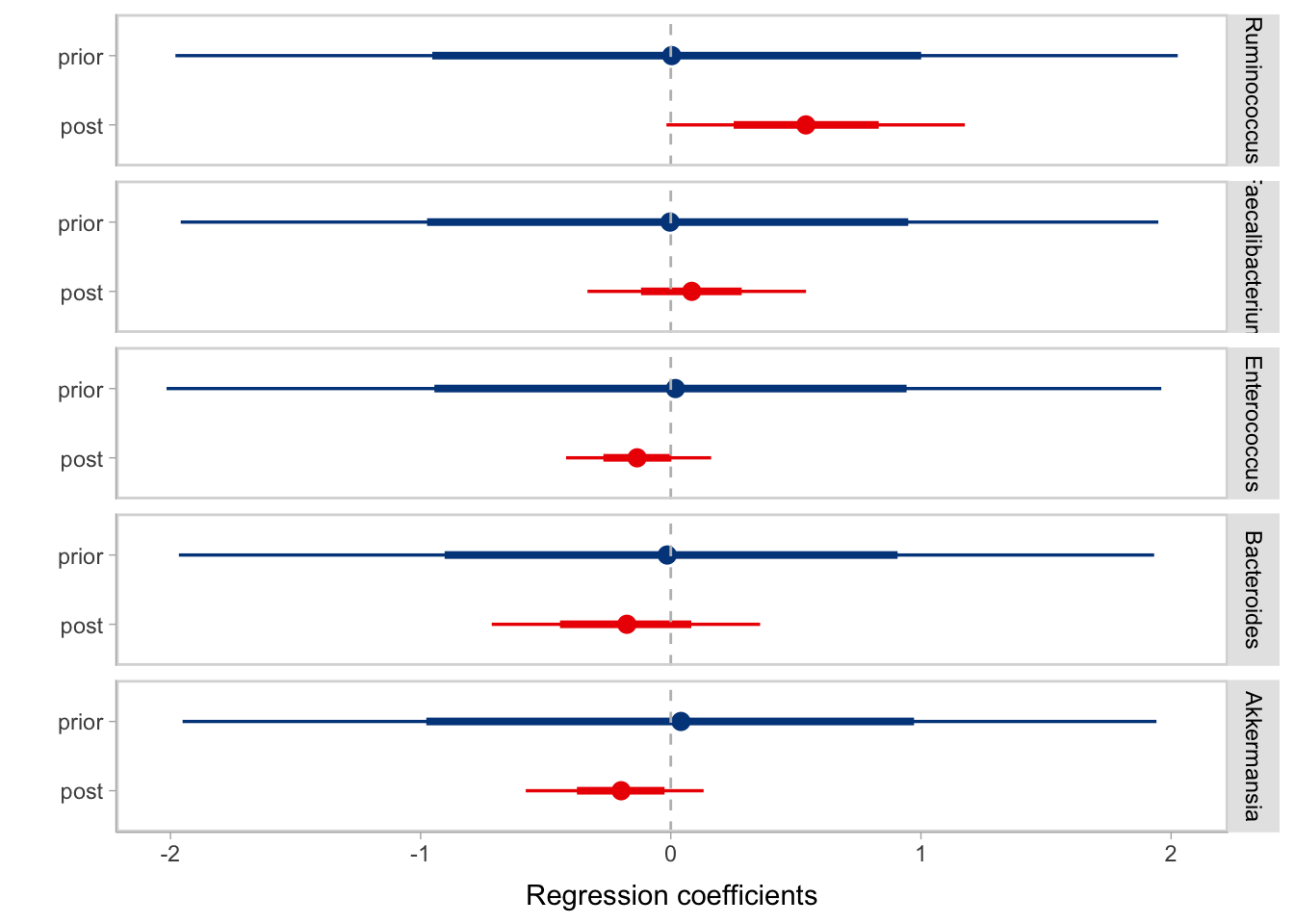
- The above figure shows the distribution of the prior coefficients as blue lines and posterior ones as red lines, both with thicker lines to denote 66% CI and thinner lines for the 95% CI. It is observed from the figure that in our prior assumption we don’t expect positive or negative correlation between taxa and CR response on average. However after learning from the data the model informed us that it is very likely Ruminococcus is positively associated with CR.
2.6 Fig3H Histogram to illustrate the predicted probability of day100 CR
post <- extract.samples(gcr)

meta_ <- meta %>%
  select(Akkermansia:Ruminococcus)

# the post coeffs in df format
postdf <- bind_cols(ba = post$ba, bb = post$bb, be = post$be, bf = post$bf, br = post$br, am = post$a[,1])

# use the 90% and 10% quantile patient data in terms of ruminococcus relab
N <- 100
# for the top and bottom quantile range of ruminococcus relab
ru_top <- meta_ %>%
  filter(Ruminococcus >= quantile(meta$Ruminococcus, 0.9))
ru_bot <- meta_ %>%
  filter(Ruminococcus <= quantile(meta$Ruminococcus, 0.1))


# a function to calculate the predicted probability with the randomly drawn coeff from the posterior distributionn and the log10 transformed relative abundance
per_pt_sample_post_prob <- function(lga_, lgb_, lge_, lgf_ , lgr_){
  # the input is the log relab of the 5 genera for that patient
  post_samp <- postdf %>%
    sample_n(size = N, replace = F)

  ret = pmap(post_samp, function(ba, bb, be, bf, br, am) {
    inv_logit( ba * lga_ + bb * lgb_ + be * lge_ +  bf * lgf_ + br * lgr_ + am )
  }) %>%
    set_names(seq(1, N)) %>%
    bind_rows() %>%
    gather()
  return(ret)
}

# for the top quantile patients
res_top <- pmap(ru_top, function(Akkermansia, Bacteroides, Enterococcus, Faecalibacterium, Ruminococcus){
  per_pt_sample_post_prob(Akkermansia, Bacteroides, Enterococcus, Faecalibacterium, Ruminococcus)
}) %>%
  set_names(paste('P', seq(1, nrow(ru_top)), sep = '')) %>%
  bind_rows(.id = 'pt')

# for the bottom quantile patients
res_bot <- pmap(ru_bot, function(Akkermansia, Bacteroides, Enterococcus, Faecalibacterium, Ruminococcus){
  per_pt_sample_post_prob(Akkermansia, Bacteroides, Enterococcus, Faecalibacterium, Ruminococcus)
}) %>%
  set_names(paste('P', seq(1, nrow(ru_bot)), sep = '')) %>%
  bind_rows(.id = 'pt')

# plot them together in one
Ruminococcus <- bind_rows(
  res_top %>% mutate(grp = 'high Ruminococcus'),
  res_bot %>% mutate(grp = 'low Ruminococcus')
) %>%
  gghistogram(x = 'value',bins = 30, fill = 'grp', palette = 'nejm', color = 'white', add = 'mean',
                  xlab = 'Predicted probability of CR d100', ylab = 'Probability density')
Ruminococcus 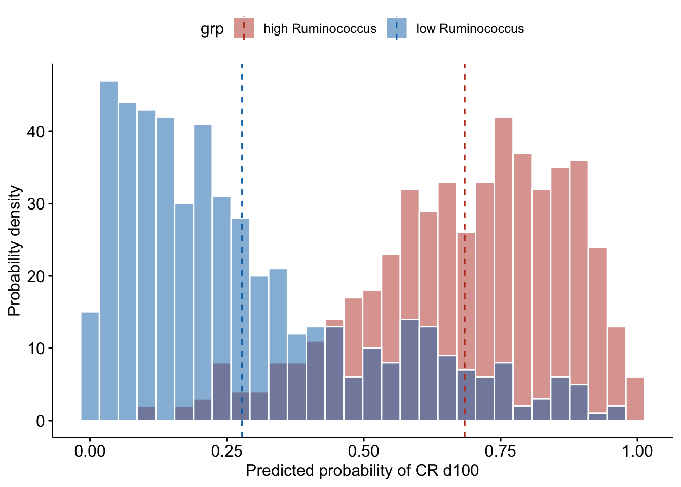
ggsave('figs/predicted_CR_Ruminococcus_top_bottom_10.pdf', width = 7, height = 5, plot = Ruminococcus)

bind_rows(
  res_top %>% mutate(grp = 'high Ruminococcus'),
  res_bot %>% mutate(grp = 'low Ruminococcus')
)  %>%
  group_by(grp) %>%
  summarise(ave = mean(value))
## # A tibble: 2 × 2
## grp ave
## <chr> <dbl>
## 1 high Ruminococcus 0.685
## 2 low Ruminococcus 0.278As can be observed from the histogram, when the patients have high Ruminococcus content (relative abundance in the top 10% of the current patient cohort), they are predicted to have on average a probability of 0.67 to have CR at day 100; whereas when they have low Ruminococcus content (relative abundance in the bottom 10% of the current patient cohort), they are predicted to have only on average a probability of 0.27 to have CR at day 100.
2.7 Fig 3I Bayesian modeling with 5 genera abundance as predictor(outcome toxicity)
Toxicity ~ Akkermansia + Bacteroides + Enterococcus + Faecalibacterium + Ruminococcus + center
gtox <- ulam(
    alist(
        tox ~ dbinom( 1 , p ) ,
        logit(p) <- ba*Akkermansia + bb*Bacteroides + be*Enterococcus + bf*Faecalibacterium + br*Ruminococcus + a[location] ,
        ba ~ dnorm( 0 , 1),
        bb ~ dnorm( 0 , 1),
        be ~ dnorm( 0 , 1),
        bf ~ dnorm( 0 , 1),
        br ~ dnorm( 0 , 1),
        a[location] ~ dnorm( 0 , 0.5 )
    ) , data=dat_list , chains=4 , log_lik=TRUE , cores = 16)
## Running /Library/Frameworks/R.framework/Resources/bin/R CMD SHLIB foo.c
## clang -mmacosx-version-min=10.13 -I"/Library/Frameworks/R.framework/Resources/include" -DNDEBUG -I"/Library/Frameworks/R.framework/Versions/4.1/Resources/library/Rcpp/include/" -I"/Library/Frameworks/R.framework/Versions/4.1/Resources/library/RcppEigen/include/" -I"/Library/Frameworks/R.framework/Versions/4.1/Resources/library/RcppEigen/include/unsupported" -I"/Library/Frameworks/R.framework/Versions/4.1/Resources/library/BH/include" -I"/Library/Frameworks/R.framework/Versions/4.1/Resources/library/StanHeaders/include/src/" -I"/Library/Frameworks/R.framework/Versions/4.1/Resources/library/StanHeaders/include/" -I"/Library/Frameworks/R.framework/Versions/4.1/Resources/library/RcppParallel/include/" -I"/Library/Frameworks/R.framework/Versions/4.1/Resources/library/rstan/include" -DEIGEN_NO_DEBUG -DBOOST_DISABLE_ASSERTS -DBOOST_PENDING_INTEGER_LOG2_HPP -DSTAN_THREADS -DBOOST_NO_AUTO_PTR -include '/Library/Frameworks/R.framework/Versions/4.1/Resources/library/StanHeaders/include/stan/math/prim/mat/fun/Eigen.hpp' -D_REENTRANT -DRCPP_PARALLEL_USE_TBB=1 -I/usr/local/include -fPIC -Wall -g -O2 -c foo.c -o foo.o
## In file included from <built-in>:1:
## In file included from /Library/Frameworks/R.framework/Versions/4.1/Resources/library/StanHeaders/include/stan/math/prim/mat/fun/Eigen.hpp:13:
## In file included from /Library/Frameworks/R.framework/Versions/4.1/Resources/library/RcppEigen/include/Eigen/Dense:1:
## In file included from /Library/Frameworks/R.framework/Versions/4.1/Resources/library/RcppEigen/include/Eigen/Core:88:
## /Library/Frameworks/R.framework/Versions/4.1/Resources/library/RcppEigen/include/Eigen/src/Core/util/Macros.h:628:1: error: unknown type name 'namespace'
## namespace Eigen {
## ^
## /Library/Frameworks/R.framework/Versions/4.1/Resources/library/RcppEigen/include/Eigen/src/Core/util/Macros.h:628:16: error: expected ';' after top level declarator
## namespace Eigen {
## ^
## ;
## In file included from <built-in>:1:
## In file included from /Library/Frameworks/R.framework/Versions/4.1/Resources/library/StanHeaders/include/stan/math/prim/mat/fun/Eigen.hpp:13:
## In file included from /Library/Frameworks/R.framework/Versions/4.1/Resources/library/RcppEigen/include/Eigen/Dense:1:
## /Library/Frameworks/R.framework/Versions/4.1/Resources/library/RcppEigen/include/Eigen/Core:96:10: fatal error: 'complex' file not found
## #include <complex>
## ^~~~~~~~~
## 3 errors generated.
## make: *** [foo.o] Error 1df <- precis(gtox, prob = 0.95) %>% as.tibble()
df <- df %>%
mutate(variable = c('Akkermansia', 'Bacteroides','Enterococcus','Faecalibacterium','Ruminococcus'))
#remove row number 1 (The intercept)
forest <- df %>%
ggplot(aes(x = variable, y = mean)) +
geom_point(shape = 15,
size = 4, width = 0.1,
position = "dodge", color="black") +
geom_errorbar(aes(ymin = `2.5%`,
ymax = `97.5%`),
width = 0.1,
size = 0.7,
position = "dodge", color="turquoise4") +
theme(axis.title = element_text(face = "bold")) +
xlab("Variables") + ylab("Coefficient with 95% CI") +
coord_flip(ylim = c(-1.5, 1.5)) +
geom_hline(yintercept = 0, color = "red", size = 1) +
theme(axis.title = element_text(size = 0)) +
theme(axis.text = element_text(size = 14)) +
labs(title = 'Toxicity') ## Warning: Ignoring unknown parameters: widthforest ## Warning: Width not defined. Set with `position_dodge(width = ?)`
ggsave('figs/amplicon/bayesian_genera_tox_log10.pdf', width = 5, height = 4, plot = forest)## Warning: Width not defined. Set with `position_dodge(width = ?)`Check the prior and posterior coeff distribution
theme_set(theme_tidybayes() + cowplot::panel_border())
# check the prior and posterior
prior <- extract.prior( gtox , n=4000 ) %>% as.tibble()  %>% select(-a) %>% mutate(grp = 'prior')
##
## SAMPLING FOR MODEL '7918a19a60166753261e9ae299e2ffc0' NOW (CHAIN 1).
## Chain 1:
## Chain 1: Gradient evaluation took 2.2e-05 seconds
## Chain 1: 1000 transitions using 10 leapfrog steps per transition would take 0.22 seconds.
## Chain 1: Adjust your expectations accordingly!
## Chain 1:
## Chain 1:
## Chain 1: Iteration: 1 / 8000 [ 0%] (Warmup)
## Chain 1: Iteration: 800 / 8000 [ 10%] (Warmup)
## Chain 1: Iteration: 1600 / 8000 [ 20%] (Warmup)
## Chain 1: Iteration: 2400 / 8000 [ 30%] (Warmup)
## Chain 1: Iteration: 3200 / 8000 [ 40%] (Warmup)
## Chain 1: Iteration: 4000 / 8000 [ 50%] (Warmup)
## Chain 1: Iteration: 4001 / 8000 [ 50%] (Sampling)
## Chain 1: Iteration: 4800 / 8000 [ 60%] (Sampling)
## Chain 1: Iteration: 5600 / 8000 [ 70%] (Sampling)
## Chain 1: Iteration: 6400 / 8000 [ 80%] (Sampling)
## Chain 1: Iteration: 7200 / 8000 [ 90%] (Sampling)
## Chain 1: Iteration: 8000 / 8000 [100%] (Sampling)
## Chain 1:
## Chain 1: Elapsed Time: 0.244513 seconds (Warm-up)
## Chain 1: 0.244409 seconds (Sampling)
## Chain 1: 0.488922 seconds (Total)
## Chain 1:post <- extract.samples(gtox) %>% as.tibble() %>% select(-a) %>% mutate(grp = 'post')
# comparing prior and post
tox <- bind_rows(prior, post) %>%
gather('term', 'coeff', ba:br) %>%
mutate(genus = case_when(
term == 'ba' ~ 'Akkermansia',
term == 'bb' ~ 'Bacteroides',
term == 'be' ~ 'Enterococcus',
term == 'bf' ~ 'Faecalibacterium',
term == 'br' ~ 'Ruminococcus'
))
post_order <- tox %>%
filter(grp == 'post') %>%
group_by(term, genus) %>%
summarise(q50 = median(coeff)) %>%
arrange(-q50) %>%
pull(genus)
tox %>%
mutate(genus = factor(genus, levels = post_order)) %>%
ggplot(aes(x = coeff, y = grp, color = grp)) +
stat_pointinterval(.width = c(.66, .95)) +
scale_color_manual(values = c('#EC0000','#00468B')) +
geom_vline(xintercept = 0, col = 'gray', linetype = 'dashed') +
facet_grid(genus ~ .) +
labs(x = 'Regression coefficients',
y = '') +
theme(legend.position = 'none') - The above figure shows the distribution of the prior coefficients as blue lines and posterior ones as red lines, both with thicker lines to denote 66% CI and thinner lines for the 95% CI. It is observed from the figure that in our prior assumption we don’t expect positive or negative correlation between taxa and toxicity response on average. However after learning from the data the model informed us that there is a trend of Ruminococcus’s negative association with toxicity and Bacteroides’s positive association with toxicity.
2.8 Fig3J Histogram to illustrate the predicted probability of toxicity
# extract posterior samples
post <- extract.samples(gtox)

meta_ <- meta %>%
  select(Akkermansia:Ruminococcus)

# the post coeffs in df format
postdf <- bind_cols(ba = post$ba, bb = post$bb, be = post$be, bf = post$bf, br = post$br, am = post$a[,1])

N <- 100
# for the top and bottom quantile range of Bacteroides relab (top and bottom 10%)
ba_top <- meta_ %>%
  filter(Bacteroides >= quantile(meta$Bacteroides, 0.9))
ba_bot <- meta_ %>%
  filter(Bacteroides <= quantile(meta$Bacteroides, 0.1))

# a function to calculate the predicted probability with the randomly drawn coeff from the posterior distributionn and the log10 transformed relative abundance
per_pt_sample_post_prob <- function(lga_, lgb_, lge_, lgf_ , lgr_){
  # the input is the log relab of the 5 genera for that patient
  post_samp <- postdf %>%
    sample_n(size = N, replace = F)

  ret = pmap(post_samp, function(ba, bb, be, bf, br, am) {
    inv_logit( ba * lga_ + bb * lgb_ + be * lge_ +  bf * lgf_ + br * lgr_ + am )
  }) %>%
    set_names(seq(1, N)) %>%
    bind_rows() %>%
    gather()
  return(ret)
}

# for the top quantile patients
res_top <- pmap(ba_top, function(Akkermansia, Bacteroides, Enterococcus, Faecalibacterium, Ruminococcus){
  per_pt_sample_post_prob(Akkermansia, Bacteroides, Enterococcus, Faecalibacterium, Ruminococcus)
}) %>%
  set_names(paste('P', seq(1, nrow(ba_top)), sep = '')) %>%
  bind_rows(.id = 'pt')

# for the bottom quantile patients
res_bot <- pmap(ba_bot, function(Akkermansia, Bacteroides, Enterococcus, Faecalibacterium, Ruminococcus){
  per_pt_sample_post_prob(Akkermansia, Bacteroides, Enterococcus, Faecalibacterium, Ruminococcus)
}) %>%
  set_names(paste('P', seq(1, nrow(ba_bot)), sep = '')) %>%
  bind_rows(.id = 'pt')

# plot them together in one
bacteroides <- bind_rows(
  res_top %>% mutate(grp = 'top'),
  res_bot %>% mutate(grp = 'bot')
) %>%
  gghistogram(x = 'value',bins = 30, fill = 'grp', palette = 'nejm', color = 'white', add = 'mean',
                  xlab = 'Predicted probability of Toxicity', ylab = 'Probability density')
bacteroides 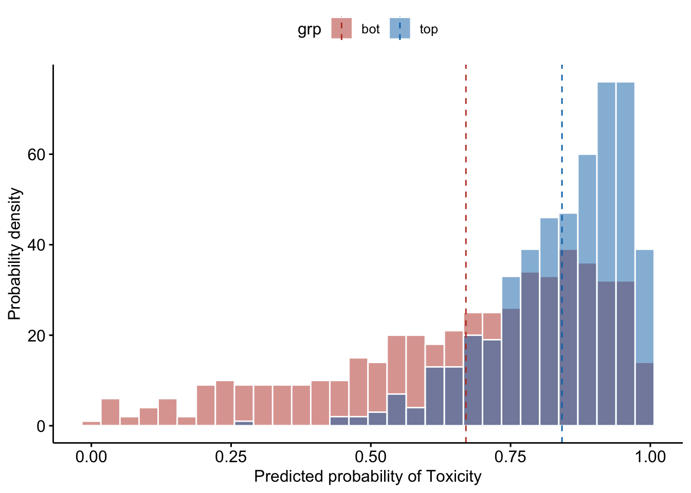
ggsave('figs/predicted_tox_bacteroides_top_bottom_10.pdf', width = 7, height = 5, plot = bacteroides)As can be observed from the histogram, when the patients have high Bacteroides content (relative abundance in the top 10% of the current patient cohort), they are predicted to almost always have a toxicity response: the histogram amassed on the right side of 0.5; whereas when the patients have low Bacteroides content (relative abundance in the bottom 10% of the current patient cohort), the patients are predicted to have no inclination towards whether or not to have a toxicity response.
2.9 Fig 3K lefse of pathway abundance using shotgun data
simple <- read_csv('data/shotgun/final_comprehensive_UPDATED_simple.csv')

pheno <- simple %>%
  gather('pheno', 'value', cr_d100:toxicity)

# the pathway counts table
full <- read_tsv('data/shotgun/humann3_pathabundance_cpm_joined_unstratified.tsv')  %>%
  rename_all(funs(str_replace(., '^CART_','')))  %>%
  rename_all(funs(str_replace(., '_humann3$','')))
## Warning: `funs()` was deprecated in dplyr 0.8.0.
## Please use a list of either functions or lambdas:
##
## # Simple named list:
## list(mean = mean, median = median)
##
## # Auto named with `tibble::lst()`:
## tibble::lst(mean, median)
##
## # Using lambdas
## list(~ mean(., trim = .2), ~ median(., na.rm = TRUE))all_sub_pheno <- pheno %>%
split(., list(.$pheno)) %>%
purrr::imap(~ filter(.data = ., value != 'not_assessed'))
all_sub_pheno %>%
imap(function(.x, .y){
select(.data = .x, value) %>%
t() %>%
write.table(str_glue('data/shotgun/pull_{.y}.txt'), sep = '\t', quote = F, row.names = T, col.names = F)
})## $cr_d100
## NULL
##
## $toxicity
## NULLall_pcts <- all_sub_pheno %>%
purrr::map(~ pull(.data = ., fid) ) %>%
imap(~ full %>% select(`# Pathway`, matches(.x)) %>%
write_tsv(str_glue('data/shotgun/pull_{.y}_pcts.tsv')))
# then move to Snakemake do the normalization and the split# add a filtering step here
# 50 and 25%
pcts <- read_tsv('data/shotgun/pull_cr_d100_pcts_cpm_unstratified.tsv') %>%
gather('sampleid', 'cpm', names(.)[2]:names(.)[ncol(.)]) %>%
rename(pw = `# Pathway`)
keeppw <- pcts %>%
filter(cpm > 50) %>%
ungroup() %>%
count(pw) %>%
filter(n > floor(nrow(simple) * 0.25)) %>%
pull(pw)
cts_fil <- pcts %>%
filter(pw %in% keeppw) %>%
spread('sampleid', 'cpm', fill = 0)
cts_fil %>%
write_tsv('data/shotgun/pull_cr_d100_pcts_cpm_unstratified_fil.tsv')# tox
pcts <- read_tsv('data/shotgun/pull_toxicity_pcts_cpm_unstratified.tsv') %>%
gather('sampleid', 'cpm', names(.)[2]:names(.)[ncol(.)]) %>%
rename(pw = `# Pathway`)
keeppw <- pcts %>%
filter(cpm > 50) %>%
ungroup() %>%
count(pw) %>%
filter(n > floor(nrow(simple) * 0.25)) %>%
pull(pw)
cts_fil <- pcts %>%
filter(pw %in% keeppw) %>%
spread('sampleid', 'cpm', fill = 0)
cts_fil %>%
write_tsv('data/shotgun/pull_toxicity_pcts_cpm_unstratified_fil.tsv')# PATHWAY
# I already normalized the pcts so don't need to normalize again here
fns <- list.files('data/shotgun/', pattern = 'lefse_ready_pcts.tsv$')
cmds <- tibble(
fns = fns
) %>%
mutate(format_cmd = str_glue('lefse_format_input.py {fns} {fns}.in -c 1 -u 2')) %>%
mutate(run_cmd = str_glue('lefse_run.py {fns}.in {fns}.res')) %>%
mutate(plot_cmd = str_glue('lefse_plot_res.py {fns}.res {fns}.pdf --format pdf --feature_font_size 4 --width 10 --dpi 300 --title {fns}')) %>%
select(-fns) %>%
gather() %>%
select(value) %>%
write_csv('data/shotgun/lefse_run_cmd.sh', col_names = F)# look at the pathway results
library(vdbR)
connect_database('~/dbConfig.txt')
get_table_from_database('metacyc_pathway_name')
get_table_from_database('metacyc_pathway_ontology')
fns <- list.files('data/shotgun/', pattern = 'lefse_ready_pcts.tsv.res$', full.names = T)
feature <- fns %>%
set_names(fns) %>%
purrr::map(~ read_tsv(., col_names = c('pathway','xx','direction','score','pval')) %>%
filter(!is.na(score))) %>%
bind_rows(.id = 'group') %>%
mutate(group = str_replace(group, 'data/shotgun//','')) %>%
mutate(group = str_replace(group, '_lefse_ready_pcts.tsv.res$',''))
# change the "N" direction to be minus score
feature <- bind_rows(
feature %>%
split(.$direction) %>%
pluck('no') %>%
mutate(score = -score),
feature %>%
split(.$direction) %>%
pluck('yes')
) %>%
arrange(group, pathway, score) %>%
mutate(pwid = str_extract(pathway, '^.+_PWY|^PWY.*_\\d{3,4}')) %>%
mutate(pwid = str_replace_all(pwid, '_', '-')) %>%
mutate(pwid = if_else(str_detect(pathway, '^TCA'), 'TCA', pwid)) %>%
mutate(pwid = if_else(str_detect(pathway, '^NAD'), 'NAD-BIOSYNTHESIS-II', pwid)) %>%
inner_join(metacyc_pathway_name %>% select(pwid, pw_name)) %>%
inner_join(metacyc_pathway_ontology %>% select(pwid, l4:l9))
all_title_fs <- 20
axis_text_fs <- 16
CR <- feature %>%
filter(group == 'pull_cr_d100') %>%
ggplot(aes(x = reorder(pathway, score), y = score, fill = direction)) +
geom_bar( stat = 'identity') +
coord_flip() +
scale_color_manual(values = c('#925E9F', '#42B540')) +
scale_fill_manual(values = c('#925E9F', '#42B540')) +
theme_classic() +
theme(axis.title.y = element_blank(),
plot.title = element_text(size=all_title_fs),
axis.title.x = element_text(size=axis_text_fs),
axis.text.x = element_text(size=axis_text_fs),
legend.position='bottom') +
labs(title = str_glue('Response to CR') ,
y = 'Score')
CR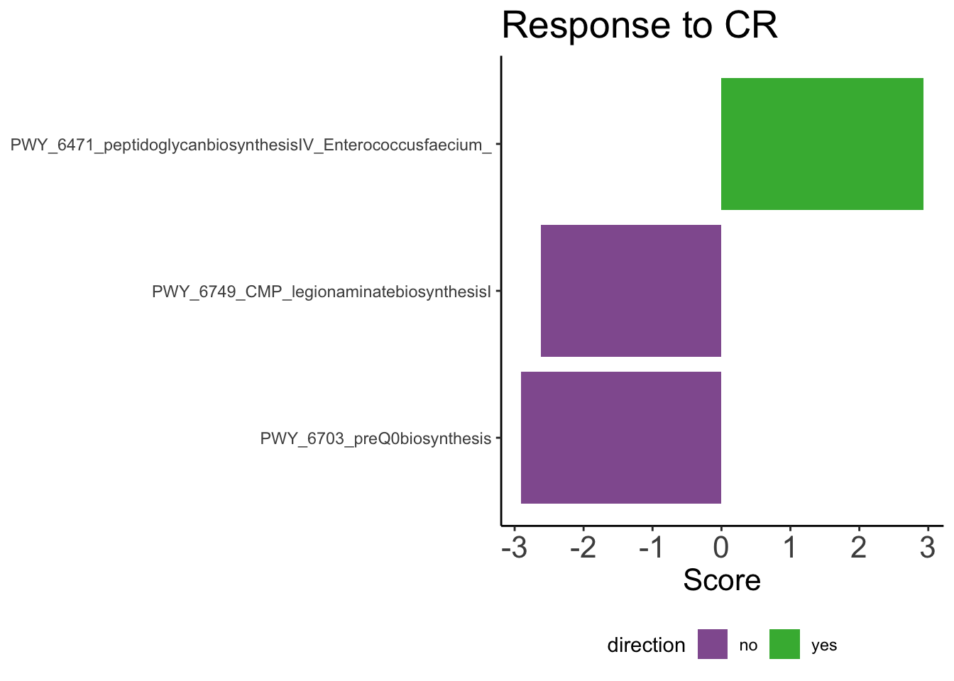
tox <- feature %>%
  filter(group == 'pull_toxicity') %>%
  ggplot(aes(x = reorder(pathway, score), y = score, fill = direction)) +
            geom_bar(stat = 'identity') +
            coord_flip() +
            scale_color_manual(values = c('#0099B4', '#AD002A'))  +
            scale_fill_manual(values = c('#0099B4', '#AD002A')) +
            theme_classic() +
            theme(axis.title.y  = element_blank(),
                  axis.title.x = element_text(size=axis_text_fs),
                  plot.title = element_text(size=all_title_fs),
                  axis.text.x = element_text(size=axis_text_fs),
                  legend.position="bottom") +
            labs(title = str_glue('Response to Toxicity') ,
                 y = 'Score')
tox
g <- cowplot::plot_grid(CR,tox,
          nrow = 2,
          rel_heights = c(1,3),
          align = 'hv',
          axis = 'b')

ggsave('figs/shotgun_lefse_tox.pdf', device = 'pdf', height = 10, width = 10, plot = tox)

ggsave('figs/shotgun_lefse_CR.pdf', device = 'pdf', height = 3, width = 10, plot = CR)
send <- asv_annotation_blast_ag %>%
filter(asv_key %in% c('asv_36','asv_3','asv_27'))
send %>%
write_csv('data/three_asv.csv')sessionInfo()## R version 4.1.1 (2021-08-10)
## Platform: x86_64-apple-darwin17.0 (64-bit)
## Running under: macOS Catalina 10.15.7
##
## Matrix products: default
## BLAS: /Library/Frameworks/R.framework/Versions/4.1/Resources/lib/libRblas.0.dylib
## LAPACK: /Library/Frameworks/R.framework/Versions/4.1/Resources/lib/libRlapack.dylib
##
## locale:
## [1] en_US.UTF-8/en_US.UTF-8/en_US.UTF-8/C/en_US.UTF-8/en_US.UTF-8
##
## attached base packages:
## [1] parallel stats graphics grDevices utils datasets methods
## [8] base
##
## other attached packages:
## [1] tidybayes_3.0.1 rethinking_2.13 rstan_2.21.2
## [4] StanHeaders_2.21.0-7 vegan_2.5-7 lattice_0.20-44
## [7] permute_0.9-5 ggpubr_0.4.0 vdbR_0.0.0.9000
## [10] RPostgreSQL_0.6-2 DBI_1.1.1 Rtsne_0.15
## [13] ape_5.5 labdsv_2.0-1 mgcv_1.8-36
## [16] nlme_3.1-152 data.table_1.14.0 forcats_0.5.1
## [19] stringr_1.4.0 dplyr_1.0.7 purrr_0.3.4
## [22] readr_2.0.1 tidyr_1.1.3 tibble_3.1.4
## [25] ggplot2_3.3.5 tidyverse_1.3.1
##
## loaded via a namespace (and not attached):
## [1] colorspace_2.0-2 ggsignif_0.6.2 ellipsis_0.3.2
## [4] rio_0.5.27 fs_1.5.0 rstudioapi_0.13
## [7] farver_2.1.0 svUnit_1.0.6 bit64_4.0.5
## [10] mvtnorm_1.1-2 fansi_0.5.0 lubridate_1.7.10
## [13] xml2_1.3.2 codetools_0.2-18 splines_4.1.1
## [16] knitr_1.33 jsonlite_1.7.2 broom_0.7.9
## [19] cluster_2.1.2 dbplyr_2.1.1 ggdist_3.0.0
## [22] compiler_4.1.1 httr_1.4.2 backports_1.2.1
## [25] assertthat_0.2.1 Matrix_1.3-4 fastmap_1.1.0
## [28] cli_3.0.1 htmltools_0.5.2 prettyunits_1.1.1
## [31] tools_4.1.1 coda_0.19-4 gtable_0.3.0
## [34] glue_1.4.2 posterior_1.0.1 V8_3.4.2
## [37] Rcpp_1.0.7 carData_3.0-4 cellranger_1.1.0
## [40] jquerylib_0.1.4 vctrs_0.3.8 tensorA_0.36.2
## [43] xfun_0.25 ps_1.6.0 openxlsx_4.2.4
## [46] rvest_1.0.1 lifecycle_1.0.0 rstatix_0.7.0
## [49] MASS_7.3-54 scales_1.1.1 vroom_1.5.4
## [52] hms_1.1.0 inline_0.3.19 yaml_2.2.1
## [55] curl_4.3.2 gridExtra_2.3 loo_2.4.1
## [58] sass_0.4.0 stringi_1.7.4 highr_0.9
## [61] checkmate_2.0.0 pkgbuild_1.2.0 zip_2.2.0
## [64] shape_1.4.6 matrixStats_0.60.1 rlang_0.4.11
## [67] pkgconfig_2.0.3 distributional_0.2.2 evaluate_0.14
## [70] labeling_0.4.2 cowplot_1.1.1 bit_4.0.4
## [73] tidyselect_1.1.1 processx_3.5.2 ggsci_2.9
## [76] magrittr_2.0.1 bookdown_0.24 R6_2.5.1
## [79] generics_0.1.0 pillar_1.6.2 haven_2.4.3
## [82] foreign_0.8-81 withr_2.4.2 abind_1.4-5
## [85] modelr_0.1.8 crayon_1.4.1 car_3.0-11
## [88] arrayhelpers_1.1-0 utf8_1.2.2 tzdb_0.1.2
## [91] rmarkdown_2.10 grid_4.1.1 readxl_1.3.1
## [94] callr_3.7.0 reprex_2.0.1 digest_0.6.27
## [97] RcppParallel_5.1.4 stats4_4.1.1 munsell_0.5.0
## [100] bslib_0.3.0